Download
1 / 9
90 likes | 259 Vues
The Demand for Goods. Total Demand. The Demand for Goods. Consumption ( C ). C = c 0 + c 1 Y D. The Demand for Goods. Investment is (largely) an exogenous variable Exogenous/autonomous/independent variables are not explained in our model

E N D
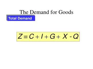
The Demand for Goods Total Demand
The Demand for Goods Consumption (C) C = c0 + c1YD
The Demand for Goods Investment is (largely) an exogenous variable • Exogenous/autonomous/independent variables are not explained in our model • Endogenous/dependent variables depend on other variables in our model C is endogenous because it responds to production: C = c0 + c1 (Y – T) • I, G & T are (largely) exogenous I = b0 + b1 Y – b2i ≈ b0 + b1 Y for now b1 = marginal propensity to invest G = G T = t0 + t1 Y t1 = marginal tax rate
The Determination ofEquilibrium Output Demand for Goods (Z) Z=c0 + c1YD + b0 + b1 Y + G = c0 + c1 (Y – T) + b0 + b1 Y + G = c0 + c1 (Y – (t0 + t1 Y)) + b0 + b1 Y + G = [c0 - c1t0 + b0 + G] + [c1 – c1 t1 + b1 ]Y = [c0 + b0 + G - c1t0 ] + [(1 - t1) c1 + b1 ]Y = Autonomous spending + Spending induced by Y
Determination of Equilibrium Output Y = Supply Z = Demand = [c0 + b0 + G - c1t0] + [(1 - t1) c1 + b1]Y Y = Z @ equilibrium Y = [c0 + b0 + G - c1t0 ] + [(1 - t1) c1 + b1 ]Y or {1 – [(1 - t1) c1 + b1 ]} Y = [c0 + b0 + G - c1t0 ] Solving for equilibrium Y Y = {1/[1 - (1 - t1) c1 - b1 ]} x [c0 + b0 + G - c1t0 ] Y = Autonomous spending multiplier x Autonomous spending When b1 = 0 and t1 = 0, Autonomous spending multiplier = 1/(1 - c1 )
The Determination ofEquilibrium Output When b1 = 0, t1 = 0, and b0 = I
Demand-Side Equilibrium and the MultiplierAt equilibrium: Y = C + I + G = ZIncrease in Y = Spending Multiplier x {Increase in Autonomous Spending}Multiplier = 1/[1 - (1 - t1) c1 - b1 ]
The Determination ofEquilibrium Output Three Steps to Solving a Model 1) Algebra to confirm the logic 2) Graphs to build the intuition 3) Words to explain the results
Determination of Equilibrium Output • The larger the marginal propensity to consume, c1, the larger the spending multiplier • The larger the propensity save (1 – c1), the less is respent, the smaller is the multiplier • A high marginal tax rate, t1, reduces the multiplier • Income leaks off into taxes and is not respent • The higher the propensity to invest as output expands, b1, the greater is the multiplier • A change in autonomous spending changes output, income and spending more than the direct change in autonomous spending