Download

1 / 85
850 likes | 1.02k Vues
Transport Layer. Motivation. What is expected out of a transport protocol for sensor networks ? Reliability, QoS (e.g., delay guarantees, priority delivery), Congestion and flow control, Energy efficiency, Fairness. Transport-Layer Challenges in WSNs.

E N D
Motivation • What is expected out of a transport protocol for sensor networks ? • Reliability, • QoS (e.g., delay guarantees, priority delivery), • Congestion and flow control, • Energy efficiency, • Fairness.
Transport-Layer Challenges in WSNs • Variety of communication models including many-to-one. • Wireless communications. • Energy constraints. • Data centric QoS. • Instead of source-destination specificic. • E.g., “provide to sink sufficient quality of information about an event”.
Motivation ..cont’d. • Application specific. • Spectra for known constraints: Low data Rate High data Rate Power limited Not Power limited Storage limited Not Storage limited Bursty samples Periodic samples
Low data Rate High data Rate Power limited Not power limited Storage limited Not storage limited user Sink Motivation ..cont’d. In general,
Trend • Departure from TCP-like model. • Relies almost exclusively on end-to-end involvement. • In general, proposed protocols engage intermediate nodes. • Transport layer? • Cross-layer approach.
Existing Solutions • Reliable delivery. • Congestion control. • Real-time scheduling.
PSFQ • Pump Slowly, Fetch Quickly. • Wan et al., ACM WSNA 2002.
Motivation • Most sensor network applications do not need 100% reliability. • Sources => sink. • But applications like re-tasking of sensors need reliable delivery. • Sink => sources. • Current sensor networks are application specific and optimized for that purpose. • Future sensor networks may be general purpose to some extent – ability to re-program functionality.
Goals • Provide lossless delivery. • Minimize control overhead. • Provide delay guarantee for delivery to all intended nodes.
Probability of successful delivery using end-to-end model 1 (1-p) 2 n-1 (1-p)n-1 n (1-p)n p is the error rate of wireless link between two hops
PSFQ’s Main Principle • “Slow” data propagation (pump). • Enough time for hop-by-hop error recovery (fetch).
1 2 3 4 1 1 1 2 2 2 3 3 3 Multi-hop packet forwarding When no link Loss – multi-hop forwarding takes place
1 3 4 2 1 1 1 2 lost 3 3 Recover 2 3 Recover 2 Recover 2 Recovering from errors Error recovery messages are wasted
1 3 4 2 1 1 2 2 lost 1 3 Recover 2 2 2 2 3 3 How PSFQ recovers from errors:“store and forward” No waste of error recovery messages
PSFQ operation • Alternate between multi-hop forwarding when low error rates and store-and-forward when error rates are higher. • 3 functions: • Pump: message relaying. • Error recovery: fetch. • Status reporting: report.
1 2 1 t Tmin 1 Tmax Tmin 1 Tmax PSFQ Pump Schedule If not duplicate and in-order and TTL not 0 then Cache and schedule for forwarding at time t (Tmin<t<Tmax)
1 2 1 1 2 2 lost 3 Tr Tr Recover 2 2 Tmin 2 Tmax “Fetch Quickly” Operation When loss detected, then fetch mode. Loss aggregation: try to recover a window of lost packets.
1 2 last-1 last Tproc last “Proactive Fetch”
Report • Report aggregation. • Carries status information: node id, seq. #. • Triggered by user. • Inject data message with “report” bit set.
Performance evaluation • Compare with SRM (Scalable Reliable Multicast) • Performance Metrics • Average Delivery Ratio • Average Latency • Average Delivery Overhead
Experimental setup 2 Mbps CSMA/CA Channel Access Tmax = 100ms Tmin = 50ms Tr = 20ms
Conclusion - PSFQ • Light weight and energy efficient • Simple mechanism • Scalable and robust • Need to be tested for high bandwidth applications • Cache size limitation
RMST • Reliable Multi-Segment Transport. • Where to do reliability? • MAC. • Transport. • Application.
MAC reliability • 802.11. • RTS/CTS, Data, Ack. • Basic stop-and-wait ARQ. • No ARQ when in broadcast or multicast modes. • Random slot selection. • Options: • No ARQ. • AEQ always. • Selective ARQ.
MAC reliability (cont’d) • Without ARQ: • Use broadcast mode. • For unicast: address screening at routing layer. • +’s: no overhead. • With ARQ: • Unicast transmissions. • For broad- & multicast, use multiple unicast. • Number of retries is configurable. • Selective ARQ: • Unicast uses ARQ. • Broad- and multicast use no ARQ. • E.g., route discovery.
Transport reliability • Strictly e2e. • Initiated by sink. • Local recovery. • Intermediate nodes trigger repair when loss is detected. • Nodes cache packets. • NACK-based.
Application-layer reliability • Directed-diffusion based. • Sink sends out request (“interest”). • When complete data received, sink removes request.
Question? • Benefits of lower-layer reliability? • Additional overhead?
RMST overview • Functions: • Fragmentation/reassembly. • Guaranteed delivery. • Unique identifiers: • “No fragments”. • Fragment id’s and number of fragments. • Loss detection and repair: • Sequence # holes and timers. • Loss detection at either sinks or intermediate nodes. • NACKs.
Preliminary analysis • Demonstrate the benefits of hop-by-hop reliability.
RMST evaluation • MAC-only reliability. • Local recovery. • With and without MAC reliability. • End-to-end reliability. • With and without MAC reliability.
Observations • When there is no transport reliability: • MAC reliability critical in lossy links. • Hop-by-hop transport reliability: • Adds little to reliable MAC. • But, hop-by-hop transport reliability only more efficient than adding MAC reliability. • MAC ARQ overhead incurred in every packet. • E2E transport reliability: • When no MAC reliability is used, simulation does not terminate: hop-by-hop recovery is critical. • If MAC reliability used, hop-by-hop and e2e transport reliability are equivalent.
Observations (cont’d) • Experiments with high error rates: • Hop-by-hop transport reliability without MAC reliability. • Hop-by-hop transport reliability+Sel. ARQ. • E2e transport reliability+ Sel. ARQ. • Hbh transport reliability without ARQ breaks down at high error rates. • Routing has hard time establishing routes.
SWSP • Simple Wireless Sensor Protocol. • Design challenges: • Limited capabilities. • Assumptions: • “Fixed network” topology. • Access points as data collectors.
Why not TCP? • Too heavy-duty. • Congestion control and wireless links. • Disable congestion control? • Low bandwidth. • Buffer size. • Small windows. • Multiple connections. • Single connection.
SWSP overview On Connecting Disconnected Power off Ack received Leave Connected Disconnecting Ack rec’d Data sent Data request Leave Ack wait Requested Data sent
Observations • Sensor registers with an AP. • Listens for RR messages. • Sends registration. • Waits for ACK => “connected” state. • Window size? • Periodic KA from sensors. • Data retransmitted after 3 retries. • ACKS piggybacked onto RR messages. • Data piggybacked onto KA messages.
SWSP evaluation • Methodology: • Platform: • PC with Linux • Simulated different sensors as different processes. • AP simulated using another PC. • Wireless communication. • Metrics: • Throughput: # of bytes received by AP/time. • Delay: time(ACK-recv’d) – time(data-sent).
SWSP evaluation (cont’d) • Throughput increases up to certain number of sensors; then decreases as sink gets overrun. • Delay increases substantially beyond a given number of sensors. • Solutions?
Congestion Control • Limited bandwidth. • Congestion is likely, e.g., when an event is detected.
S Event-to-Sink Reliable Transport (ESRT) for Wireless Sensor Networks • Akyildiz et al., ACM Mobihoc 2003 • Event-to-sink reliability. • Self-adjusting. • Energy awareness [low power consumption requirement!]. • Congestion control. • Different complexity at source and sink.
ESRT’s definition of reliability • Reliability is measured in terms of the number of packets received. Or reporting frequency i.e., number of packets/decision interval. • Observed reliability: number of received data packets in decision interval at the sink. • Desired reliability: number of packets required for reliable event detection. • Reporting rate: number of packets sent by sensor over time interval. • Normalized reliability: observed/desired.
ESRT problem definition Determine reporting frequency of source nodes to achieve required reliability at sink with minimum resource consumption.