Download
1 / 14
140 likes | 261 Vues
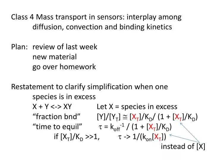
Class 4 Mass transport in sensors: interplay among diffusion, convection and binding kinetics Plan: review of last week new material go over homework Restatement to clarify simplification when one species is in excess X + Y <-> XY Let X = species in excess

E N D
Class 4 Mass transport in sensors: interplay among diffusion, convection and binding kinetics Plan: review of last week new material go over homework Restatement to clarify simplification when one species is in excess X + Y <-> XY Let X = species in excess “fraction bnd” [Y]/[YT] @[XT]/KD/ (1 + [XT]/KD) “time to equil” t = koff-1 / (1 + [XT]/KD) if [XT]/KD >>1, t -> 1/(kon[XT]) instead of [X]
Questions about binding kinetics? What did you learn from hospital lab visit? Cepheid patent on automated sample prep http://www.faqs.org/patents/app/20120171758 what was important to users lab tech lab director purchasing decision-makers
Kinetic limits on sensors imposed by rates of diffusion, convection (delivery by flow), and reaction (binding to capture molecule) Consider standard flow cell geometry Q = area (HW) x fluid velocity sensing surface Basic idea – most sensors flow sample by sensing surface If flow is slow compared to diffusion and binding, region near sensor surface gets depleted of analyte, which slows rate of detection.
Imagine what [ligand] looks like over time sensor surface time What would analytedistribution look like at equilibrium if flow was 0? We’ll focus on transient steady-state when most receptors still free to bind ligand What happens to flux to sensor surface over time Flux plotted in units of flux at time it takes ligand to diffuse H; Time in units of time it takes ligand to diffuse H
If flow is fast, portions of the sample are never “seen” by the detector. How can one match these rates for best operation in particular applications? How can one estimate analyte conc. near surface? These issues are crucial in real-time sensing (SPR) and when dealing with very low concentration analyte.
Main points to cover Relationships between flow rate Q, fluid velocity U, channel dimensions H and W, pressure P, viscosity h How big is depletion region at “low” flow rates How big is depletion region at “high” flow rates How much does depletion slow approach to equil.
Relations between flow rate Q, Width W, Height H, sensor length L, average fluid velocity U, pressure P, viscosity h, etc. Common geometry H<<W L z Q [vol/s] = area x average velocity = W H U Total flux [molec/s] = Q x c x area Fluid velocity profile is parabolic with z: u(z) = 6 U z(H-z)/H2 How would you expect Q to vary with P, W, H, L, h? ~ P W H / Lh Q= (H2/12)PWH/Lh (H<<W)
2. How big is depletion region d (roughly) at low flow rates? If flow slows, how does d change? If flow increases, how does d change? At steady state, total flux from convection Q c0 = total flux from diffusion (D (c0 – 0)/d ) H W => d = H W D / Q d/H = dimensionless (loved by fluid dynamacists!) = 1/PeH, when d >> H, PeH <<1 “PecletH ” If d << H, does this way of measuring flux make sense? No c0 d
3. How big is depletion region d at high flow rates (e)? Here conc = co at some height dabove sensor L At steady-state: time to diffuse d = time to flow over L d2/D = L/u(d) have to consider how velocity changes with height u(d) = 6Qd/WH2 ford<<H -> d/L = (DH2W/6QL2)1/3= (1/Pes)1/3 “PecletS”
4. How much does depletion slow approach to equil.? Estimate cS = conc at which rate molecules diffuse across d from c0 to cs = rate at which they bind to receptor (assume “vertical” geometry for this exercise, and calculate “initial” binding rate when all Ab’s are free; let sensor area = As and # Abs/unit area = b) JD = As x D x (c0 – cS)/dS= AsD(c0 – cS)(PeS)1/3/L JR = kon x cS x # free receptors on surface = koncS b As => cS/c0 = 1/(1 + konbL/D(PeS)1/3)= 1/(1+Da) “Damkohler” #, Da = measure of ratio between flow and binding rates when Da >> 1, cS@ c0 /Daand teq@Datrxn (slower)
We’ll use these formulas to get a sense of concentrations in (different regions within) flow cell at different flow rates and expected time to accumulate signal Caveat: these formulas apply to “continuum” model and become inappropriate when concentrations are so low that only a few ligand molecules are in sensor at any time Some articles claiming “single-molecule” sensors violate these estimates, raising questions whether they can be true (e.g. are results reproducible, do they represent selected experiments, etc.
Possible ways mass transport limits could be exceeded: Use some force to bring analyteto sensorsurface faster than diffusion (magnetic, electrophoretic, laser trap force)
Summary of useful formulas for this course xrms =(6Dt)1/2D [m2/s] D = kBT/6phr (Stokes-Einstein) kBT = 4x10-21J = 4pNnm at room temp h(viscosity) = 10-3Ns/m2 for water jD [#/(area s)] = D (Dc/Dx)(Fick) PeH = Q/WCD d/H = 1/PeH when PeH < 1 PeS= 6l2PeHl = L/H dS/L = 1/(PeS)1/3 Y/YT -> [XT/KD /(1 + XT/KD)] X = “excess” reactant trxn= koff-1/(1+ XT/KD) KD = koff/kon[M] Da = konbL/D(PeS)1/3teq = Datrxnwhen Da>1 kon typically ~104 -106/Ms for proteins Fdrag = 6phr*velocity flow between parallel plates: Q=H3WP/12hL velocity near surface = 6Qz/WH2
Next class – microscale cantilever – measure mass of captured analyte = different transduction method Basic advance – putting flow cell inside cantilever, you can operate cantilever in air or vacuum with minimal drag compared to cantilever sensors immersed in liquids Will use Manalis formulae to estimate mass transport characteristics! Read: Burg et al (from Manalis lab!) Weighing biomolecules Nature 446:1066 (2007)