Download
1 / 33
330 likes | 549 Vues
Applied Neuro-Dynamic Programming in the Game of Chess. James Gideon. Dynamic Programming (DP). Family of algorithms applied to problems where decisions are made in stages and a reward or cost is received at each stage that is additive over time Optimal control method Example:

E N D
Applied Neuro-Dynamic Programming in the Game of Chess James Gideon
Dynamic Programming (DP) • Family of algorithms applied to problems where decisions are made in stages and a reward or cost is received at each stage that is additive over time • Optimal control method • Example: Traveling Salesman Problem
Bellman’s Equation • Stochastic DP • Deterministic DP
Key Aspects of DP • Problem must be structured into overlapping sub-problems • Storage and retrieval of intermediate results is necessary (tabular method) • State space must be manageable • Objective is to calculate numerically the state value function, J*(s), and optimize the right hand side of Bellman’s equation so that the optimal decision can be made for any given state
Neuro-Dynamic Programming (NDP) • Family of algorithms applied to DP-like problems with either a very large state-space or an unknown environmental model • Sub-optimal control method • Example: Backgammon (TD-Gammon)
Key Aspects of NDP • Rather than calculating the optimal state value function, J*(s), the objective is to calculate the approximate state value function J~(s,w) • Neural Networks are used to represent J~(s,w) • Reinforcement learning is used to improve the decision making policy • Can be an on-line or off-line learning approach • The Q-Factors of the state-action value function, Q*(s,a), could be calculated or approximated (Q*(s,a,w)) instead of J~(s,w)
The Game of Chess • Played on 8x8 board with 6 types of pieces per side (8 pawns, 2 knights, 2 bishops, 2 rooks, 1 queen and 1 king) each with its own rules of movement • The two sides (black and white) alternate turns • Goal is to capture the opposing side’s king Initial Position
The Game of Chess • Very complex with approximately 1040 states and 10120 possible games • Has clearly defined rules and is easy to simulate making it an ideal problem for exploring and testing the ideas in NDP • Despite recent successes in computer chess there is still much room for improvement, particularly in learning methodologies
The Problem • Given any legal initial position choose the move leading to the largest long term reward
A Theoretical Solution • Solved with a direct implementation of the DP algorithm (a simple recursive implementation of Bellman’s Equation, e.g. the Minimax algorithm with last stage reward evaluation) • Results in an optimal solution, J*(s) • Computationally intractable (would take roughly 1035 MB of memory and 1017 centuries of calculation)
A Practical Solution • Solved with a limited look-ahead version of the Minimax algorithm with approximated last stage reward evaluation • Results in a sub-optimal solution, J~(s,w) • Useful because an arbitrary amount of time or look-ahead can be allocated to the computation of the solution
Alpha-Beta Minimax • By adding lower (alpha) and upper (beta) bounds on the possible range of scores a branch can return, based on scores from previously analyzed branches, complete branches can be removed from the look-ahead without being expanded
Alpha-Beta Minimax with Move Ordering • Works best when moves at each node are tried in a reasonably good order • Use iterative deepening look-ahead • Rather than analyzing a position at an arbitrary Minimax depth of n, analyze iteratively and incrementally at depth 1, 2, 3, …, n • Then try best move at previous iteration first in next iteration • Counter-intuitive, but very good in practice!
Alpha-Beta Minimax with Move Ordering • MVV/LVA – Most Valuable Victim, Least Valuable Attacker • First sort all capture moves based on value of capturing piece and value of captured piece then try in that order • Next try Killer Moves • Moves that have caused an alpha or beta cutoff at the current depth in a previous iteration of iterative deepening • History Moves (History Heuristic) • Finally try rest of moves based on historical results during the entire course of the iterative deepening Minimax algorithm and try in order based on “Q-Factors” (sort of)
Hash Tables • Minimax alone is not a DP algorithm because it does not reuse previously computed results • The Minimax algorithm frequently re-expands and recalculates the values of chess positions • Zobrist hashing is an efficient method of storing scores of previously analyzed positions in a table for reuse • Combined with hash tables, Minimax becomes a DP algorithm!
Minimal Window Alpha-Beta Minimax • NegaScout/PVS – Principal Variation Search • Expands decision tree with infinite alpha-beta bounds for the first move at each depth of recursion, subsequent expansions are performed with alpha, alpha+1 bounds • Works best when moves are ordered well in an iterative deepening framework • MTD(f) – Memory Enhanced Test Driver • Very sophisticated, can be thought of as a “binary search” into the decision tree space by continuously probing state-space with alpha-beta window equal to 1 and adjusting additional parameters accordingly • DP algorithm by design, requires a hash table • Works best with good first guess f and well ordered moves
Other Minimax Enhancements • Quiescence Search • At leaf positions run Minimax search to conclusion while only generating capture moves at each position • Avoids a n-ply look-ahead from terminating in the middle of a capture sequence and misevaluating the leaf position • Results in increased accuracy of the position evaluation, J~(s,w)
Other Minimax Enhancements • Null-Move Forward Pruning • During certain positions in the decision tree let the current player “pass” the move to the other player, perform Minimax algorithm at a reduced look-ahead, then if score returned is still greater than the upper bound it is assumed that if the current player had actually moved then the resulting Minima score would still be greater than the upper bound, so take the beta cutoff immediately • Results in excellent reduction of nodes expanded in the decision tree
Other Minimax Enhancements • Selective Extensions • At “interesting” positions in the decision tree extend the look-ahead by additional stages • Futility Pruning • Based on alpha-beta values at leaf nodes it can sometimes be reasonably assumed that if the quiescence look-ahead was run it would still return a result lower than alpha, so take an alpha cutoff immediately
Evaluating a Position • The approximate state (position) value function, J~(s,w), can be approximated with a “smoother” feature value function J~(f(s),w) where f(s) is the function that maps states into feature vectors • Process is called feature extraction • Could also calculate the approximate state-feature value function J~(s,f(s),w)
Evaluating a Position • Most chess systems use only approximate DP when implementing the decision making policy, that is the weight vector w of J~(-,w) is predefined and constant • In a true NDP implementation the weight vector w is adjusted through reinforcements to improve the decision making policy
General Positional Evaluation Architecture • White Approximator • Fully connected MLP neural network • Inputs of state and feature vectors specific to white • One output indicating favorability (+/-) of white positional structure • Black Approximator • Fully connected MLP neural network • Inputs of state and feature vectors specific to black • One output indicating favorability (+/-) of black positional structure • Final output is the difference between both network outputs
Material Balance Evaluation Architecture • Two simple linear tabular evaluators, one for white and one for black
Pawn Structure Evaluation Architecture • White Approximator • Fully connected MLP neural network • Inputs of state and feature vectors specific to white • One output indicating favorability (+/-) of white positional structure • Black Approximator • Fully connected MLP neural network • Inputs of state and feature vectors specific to black • One output indicating favorability (+/-) of black positional structure • Final output is the difference between both network outputs
The Learning Algorithm • Reinforcement learning method • Temporal difference learning • Use difference of two time successive approximations of position value to adjust the weights of neural networks • Value of final position is a value suitably representative of the outcome of the game
The Learning Algorithm • TD(λ) • Algorithm that applies the temporal difference error correction to decisions arbitrarily far back in time discounted by a factor of λ at each stage • λ must be in the interval [0,1]
The Learning Algorithm • Presentation of training samples is provided by the TDLeaf(λ) algorithm (uses look-ahead evaluation for training targets) • Weights for all networks are adjusted according to Backpropagation algorithm Neuron j output Neuron j local field
Self Play Training vs. On-Line Play Training • In self play simulation the system will play itself to train the position evaluator neural networks • Policy of move selection should randomly select non-greedy actions a small percentage of the time so that there is a non-zero probability of exploring all actions (e.g. the Epsilon-Greedy algorithm) • System can be fully trained before deployment
Self Play Training vs. On-Line Play Training • In on-line play the system will play other opponents to train the position evaluator neural networks • Requires no randomization of the decision making policy since opponent will provide sufficient exploration of the state-space • System will be untrained initially at deployment