Download
1 / 77
780 likes | 971 Vues
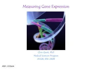
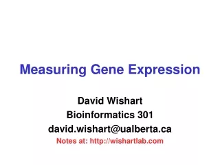
Measuring Gene Expression Part 3. David Wishart Bioinformatics 301 david.wishart@ualberta.ca. Objectives*. Become aware of some of the causes of low quality microarray data Become familiar with gridding, spot picking, intensity determination & quality control issues

E N D
Measuring Gene Expression Part 3 David Wishart Bioinformatics 301 david.wishart@ualberta.ca
Objectives* • Become aware of some of the causes of low quality microarray data • Become familiar with gridding, spot picking, intensity determination & quality control issues • Become familiar with normalization, curve fitting and correlation • Understand how microarray data is analyzed
Key Steps in Microarray Analysis* • Quality Control (checking microarrays for errors or problems) • Image Processing • Gridding • Segmentation (peak picking) • Data Extraction (intensity, QC) • Data Analysis and Data Mining
Comet Tailing* • Often caused by insufficiently rapid immersion of the slides in the succinic anhydride blocking solution.
Uneven Spotting/Blotting • Problems with print tips or with overly viscous solution • Problems with humidity in spottiing chamber
Gridding Errors Spotting errors Uneven hybridization Gridding errors
Key Steps in Microarray Analysis • Quality Control (checking microarrays for errors or problems) • Image Processing • Gridding • Segmentation (spot picking) • Data Extraction (intensity, QC) • Data Analysis and Data Mining
PMT Pinhole Detector lens Laser Beam-splitter Objective Lens Dye Glass Slide Microarray Scanning*
Microarray Principles* Laser 1 Laser 2 Green channel Red channel Scan and detect with confocal laser system overlay images and normalize Image process and analyze
Microarray Images • Resolution • standard 10m [currently, max 5m] • 100m spot on chip = 10 pixels in diameter • Image format • TIFF (tagged image file format) 16 bit (64K grey levels) • 1cm x 1cm image at 16 bit = 2Mb (uncompressed) • other formats exist i.e. SCN (Stanford University) • Separate image for each fluorescent sample • channel 1, channel 2, etc.
Image Processing* • Addressing or gridding • Assigning coordinates to each of the spots • Segmentation or spot picking • Classifying pixels either as foreground or as background • Intensity extraction (for each spot) • Foreground fluorescence intensity pairs (R, G) • Background intensities • Quality measures
Gridding Considerations* • Separation between rows and columns of grids • Individual translation of grids • Separation between rows and columns of spots within each grid • Small individual translation of spots • Overall position of the array in the image • Automated & manual methods available
Spot Picking • Classification of pixels as foreground or background (fluorescence intensities determined for each spot are a measure of transcript abundance) • Large selection of methods available, each has strengths & weaknesses
Fixed circle ScanAlyze, GenePix, QuantArray Adaptive circle GenePix, Dapple Adaptive shape Spot, region growing and watershed Histogram method ImaGene, QuantArraym DeArray and adaptive thresholding Spot Picking* • Segmentation/spot picking methods: • Fixed circle segmentation • Adaptive circle segmentation • Adaptive shape segmentation • Histogram segmentation
GenePix finds spots by detecting edges of spots (second derivative) Adaptive Circle Segmentation* • The circle diameter is estimated separately for each spot • Problematic if spot exhibits oval shapes
Information Extraction • Spot Intensities • mean (pixel intensities) • median (pixel intensities) • Background values • Local Background • Morphological opening • Constant (global) • Quality Information Take the average
Spot Intensity* • The total amount of hybridization for a spot is proportional to the total fluorescence at the spot • Spot intensity = sum of pixel intensities within the spot mask • Since later calculations are based on ratios between cy5 and cy3, we compute the average* pixel value over the spot mask • Can use ratios of medians instead of means
Means vs. Medians* etc.
Mean, Median & Mode Mode Median Mean
Mean, Median, Mode* • In a Normal Distribution the mean, mode and median are all equal • In skewed distributions they are unequal • Mean - average value, affected by extreme values in the distribution • Median - the “middlemost” value, usually half way between the mode and the mean • Mode - most common value
Background Intensity • A spot’s measured intensity includes a contribution of non-specific hybridization and other chemicals on the glass • Fluorescence intensity from regions not occupied by DNA can be different from regions occupied by DNA
ScanAlyze ImaGene Spot, GenePix Local Background Methods* • Focuses on small regions around spot mask • Determine median pixel values in this region • Most common approach • By not considering the pixels immediately surrounding the spots, the background estimate is less sensitive to the performance of the segmentation procedure
Quality Measurements* • Array • Correlation between spot intensities • Percentage of spots with no signals • Distribution of spot signal area • Inter-array consistency • Spot • Signal / Noise ratio • Variation in pixel intensities • ID of “bad spots” (spots with no signal)
Cy5 (red) intensity Cy3 (green) intensity A Microarray Scatter Plot
Cy5 (red) intensity Cy3 (green) intensity Correlation* Comet-tailing from non- balanced channels Cy5 (red) intensity Cy3 (green) intensity Linear Non-linear
Correlation “+” correlation Uncorrelated “-” correlation
Correlation High correlation Low correlation Perfect correlation
S(xi - mx)(yi - my) r = S(xi - mx)2(yi - my)2 Correlation Coefficient* r = 0.85 r = 0.4 r = 1.0
Correlation Coefficient • Sometimes called coefficient of linear correlation or Pearson product-moment correlation coefficient • A quantitative way of determining what model (or equation or type of line) best fits a set of data • Commonly used to assess most kinds of predictions or simulations
Correlation and Outliers Experimental error or something important? A single “bad” point can destroy a good correlation
Outliers* • Can be both “good” and “bad” • When modeling data -- you don’t like to see outliers (suggests the model is bad) • Often a good indicator of experimental or measurement errors -- only you can know! • When plotting gel or microarray expression data you do like to see outliers • A good indicator of something significant
Why Log2 Transformation?* • Makes variation of intensities and ratios of intensities more independent of absolute magnitude • Makes normalization additive • Evens out highly skewed distributions • Gives more realistic sense of variation • Approximates normal distribution • Treats up- and down- regulated genes symmetrically
Log Transformations Applying a log transformation makes the variance and offset more proportionate along the entire graph 16 log2 ch2 intensity ch1ch2ch1/ch2 60 000 40 000 1.5 3000 2000 1.5 log2 ch1log2 ch2log2 ratio 15.87 15.29 0.58 11.55 10.97 0.58 0 log2 ch1 intensity 16
exp’t B linear scale exp’t B log transformed Log Transformation
Normalization* • Reduces systematic (multiplicative) differences between two channels of a single hybridization or differences between hybridizations • Several Methods: • Global mean method • (Iterative) linear regression method • Curvilinear methods (e.g. loess) • Variance model methods Try to get a slope ~1 and a correlation of ~1
1) 2) Example Where Normalization is Needed
1) 2) Example Where Normalization is Not Needed
Normalization to a Global Mean* • Calculate mean intensity of all spots in ch1 and ch2 • e.g. ch2 = 25 000 ch2/ch1 = 1.25 • ch1 = 20 000 • On average, spots in ch2 are 1.25X brighter than spots in ch1 • To normalize, multiply spots in ch1 by 1.25
Visual Example: Ch2 is too Strong Ch 1 Ch 2 Ch1 + Ch2
Visual Example: Ch2 and Ch1 are Balanced Ch 1 Ch 2 Ch1 + Ch2
Pre-normalized Data y = x + 0.84 ch2 log2 signal intensity y = x log(ch1 ) = 10.88 log(ch2 ) = 11.72 log(ch2 - ch1)= 0.84 ch1 log2 signal intensity
y = (x) (x)= x + 0.84 ch2 log2 signal intensity y = x Add 0.84 to every value in ch1 to normalize ch1 log2 signal intensity Normalized Microarray Data
Normalization to Loess Curve* • A curvilinear form of normalization • For each spot, plot ratio vs. mean (ch1,ch2) signal in log scale (A vs. M) • Use statistical programs (e.g. S-plus, SAS, or R) to fit a loess curve (local regression) through the data • Offset from this curve is the normalized expression ratio
The A versus M Plot* More Informative Graph M = log2 (R/G) A = 1/2 log2 (R*G)