Download
1 / 29
290 likes | 490 Vues
Numerical Methods for Engineering MECN 3500. Professor: Dr. Omar E. Meza Castillo omeza@bayamon.inter.edu http://www.bc.inter.edu/facultad/omeza Department of Mechanical Engineering Inter American University of Puerto Rico Bayamon Campus. Tentative Lectures Schedule.

E N D
Numerical Methods for Engineering MECN 3500 Professor: Dr. Omar E. Meza Castillo omeza@bayamon.inter.edu http://www.bc.inter.edu/facultad/omeza Department of Mechanical Engineering Inter American University of Puerto Rico Bayamon Campus
Approximations and Round-Off Errors Accuracy and Precision
Course Objectives • To understand the concept of error and its importance to the effective use of numerical methods.
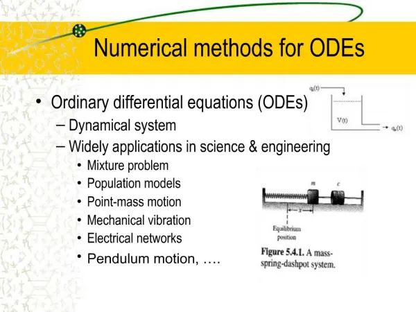
Introduction • For many engineering problems, we cannot obtain analytical solutions. • Numerical methods yield approximate results, results that are close to the exact analytical solution. We cannot exactly compute the errors associated with numerical methods. • Only rarely given data are exact, since they originate from measurements. Therefore there is probably error in the input information. • Algorithm itself usually introduces errors as well, e.g., unavoidable round-offs, etc … • The output information will then contain error from both of these sources. • How confident we are in our approximate result? • The question is “how much error is present in our calculation and is it tolerable?”
Accuracy and Precision • Accuracy. How close is a computed or measured value to the true value • Precision (or reproducibility). How close is a computed or measured value to previously computed or measured values. • Inaccuracy(or bias). A systematic deviation from the actual value. • Imprecision(or uncertainty). Magnitude of scatter.
Significant Figures • Number of significant figures indicates precision. Significant digits of a number are those that can be used with confidence, e.g.,the number of certain digits plus one estimated digit. 53,800 How many significant figures? 5.38 x 1043 5.380 x 1044 5.3800 x 1045 • Zeros are sometimes used to locate the decimal point not significant figures. 0.00001753 4 0.0001753 4 0.001753 4
True Value = Approximation + Error Et = True value – Approximation (+/-) Error Definitions True error
Error Definitions Example 3.1: Calculation of Errors • Problem Statement: Suppose that you have the task of measuring the lengths of a bridge and a rivet and come up with 9999 and 9 cm, respectively. If the true values are 10000 and 10 cm, respectively, compute (a) the true error and (b) the true percent relative error for each case. • Solution: The error for measuring the bridge Et=10000-9999=1cm And for the rivet it is Et=10-9=1cm
Error Definitions The percent relative error for the bridge is And for the rivet it is • Thus, although both measurements have an error of 1 cm, the relative error for the rivet is much greater.
Error Definitions • For numerical methods, the true value will be known only when we deal with functions that can be solved analytically (simple systems). In real world applications, we usually not know the answer a priori. Then • Iterative approach, example Newton’s method (+ / -)
Error Definitions • Use absolute value. • Computations are repeated until stopping criterion is satisfied. • If the following Scarborough criterion is met • you can be sure that the result is correct to at least n significant figures. Pre-specified % tolerance based on the knowledge of your solution
Error Definitions Example 3.2: Error Estimates for Iterative Methods • Problem Statement: In mathematics, functions can often be represented by infinite series. For example, the exponential function can be computed using Maclaurin Series Expansion. Starting with the simplest version, ex=1, add terms one at a time to estimate e0.5. Note that the true value e0.5= 1.648721 • Solution:
Error Definitions • First to determine the error criterion that ensures a result is correct to at least three significant figures: • First term • The True error: Et= 1.648721 – 1= 0.648721
Error Definitions • Second term • The True error: Et= 1.648721 – 1.5= 0.148721
Error Definitions • The entire computation can be summarized as • Thus, after the six terms are included, the approximate error falls below εs=0.05% and the computation is terminated
Round-Off Error • Round-off errors originate from the fact that computers retain only a fixed number of significant figures during a calculation. Number such as pi, e, or sqrt(7) cannot be expressed by a fixed number of significant figures. Therefore they cannot be represented exactly by the computer. • Computer use a base-2 representation, they can not precisely represent certain exact base-10 numbers. • The discrepancy introduced by this omission of significant figures is called round-off error.
Computer Representation of Numbers • Numerical round-off error is related to the manner in which number are stored. • “Word” is the fundamental unit of information storage. It consist of a string of binary digits or bits. • Number Systems: • Decimal-Base-10 System: 0, 1, 2, 3, 4, 5, 6, 7, 8, 9 • Binary-Base-2 System: 0, 1
Computer Representation of Numbers • Integer Representation: The previous slides show how to represent 10-based numbers to binary form. • The most straightforward approach to represent integers on a computer is called signed magnitude method. It employs the first bit of a word to indicate the sign, with o for positive and a 1 for negative. • Representation of the decimal integer -173 on a 16-bit computer.
Computer Representation of Numbers • Floating-Point Representation: Fractional quantities are typically represented in computer using floating-point form. In this approach, the number is expressed as a fractional part, called a mantissa or significand, and a integer part, called an exponent or characteristic, as in Integer part exponent mantissa Base of the number system used
Computer Representation of Numbers • 156.780.15678x103 in a floating point base-10 system.
Computer Representation of Numbers • Normalized to remove the leading zeroes. Multiply the mantissa by 10 and lower the exponent by 1. • 0.2941 x 10⁻¹ • Suppose only 4 decimal places to be stored Additional significant figure is retained
Computer Representation of Numbers Therefore for a base-10 system 0.1 ≤m<1 for a base-2 system 0.5 ≤m<1 • Floating point representation allows both fractions and very large numbers to be expressed on the computer. However, • Floating point numbers take up more room. • Take longer to process than integer numbers. • Round-off errors are introduced because mantissa holds only a finite number of significant figures.
Chopping Example: • π=3.14159265358 to be stored on a base-10 system carrying 7 significant digits. • π =3.141592 chopping error et=0.00000065 • π =3.141593 rounded error et=0.00000035 • Some machines use chopping, becauserounding adds to the computational overhead. Since number of significant figures is large enough, resulting chopping error is negligible.
Homework2 www.bc.inter.edu/facultad/omeza Omar E. Meza Castillo Ph.D.