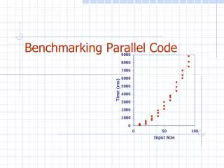
Benchmarking Parallel Code

1. Benchmarking Parallel Code

2. Benchmarking • What are the performance characteristics of a parallel code? • What should be measured? Benchmarking

3. Experimental Studies • Write a program implementing the algorithm • Run the program with inputs of varying size and composition • Use “system clock” to get an accurate measure of the actual running time • Plot the results Benchmarking

4. Experimental Dimensions • Time • Space • Number of processors • InputData(n,_,_,_) • Results(_,_) Benchmarking

5. Features of a good experiment? • What are features of every good experiment? Benchmarking

6. Features of a good experiment • Reproducibility • Quantification of performance • Exploration of anomalies • Exploration of design choices • Capacity to explain deviation from theory Benchmarking

7. Types of experiments • Time and Speedup • Scaleup • Exploration of data variation Benchmarking

8. Speedup Benchmarking

9. Time and Speedup fixed data(n,_,_,…) fixed data(n,_,_,…) linear time speedup processors processors Benchmarking

10. Superlinear Speedup • Is this possible? • Theoretical, No • What is T1? • In Practice, yes • Cache effects • “Relative Speedup” T1= parallel code on 1 process without communications fixed data(n,_,_,…) linear processors Benchmarking

11. How to lie about Speedup? • Cripple the sequential program! • This is a *very* common practice • People compare the performance of their parallel program on p processors to its performance on 1 processor, as if this told you something you care about, when in reality their parallel program on one processor runs *much* slower than the best known sequential program does. • Moral: anytime anybody shows you a speedup curve, demand to know what algorithm they're using in the numerator. Benchmarking

12. Sources of Speedup Anomalies • Reduced overhead -- some operations get cheaper because you've got fewer processes per processor • Increasing cache size -- similar to the above: memory latency appears to go down because the total aggregate cache size went up • Latency hiding -- if you have multiple processes per processor, you can do something else while waiting for a slow remote op to complete • Randomization -- simultaneous speculative pursuit of several possible paths to a solution • It should be noted that anytime "superlinear" speedup occurs for reasons 3 or 4, the sequential algorithm could (given free context switches) be made to run faster by mimicking the parallel algorithm. Benchmarking

13. Sizeup fixed p, data(_,_,…) What happens when n grows? time n Benchmarking

14. Scaleup fixed n/p, data(_,_,…) What happens when p grows, given a fixed ration n/p? time p Benchmarking

15. Exploration of data variation • Situation dependent • Let’s look at an example… Benchmarking

16. Example of Benchmarking • See http://web.cs.dal.ca/~arc/publications/1-20/paper.pdf We have implemented our optimized data partitioning method for shared-nothing data cube generation using C++ and the MPI communication library. This implementation evolved from (Chen, et.al. 2004), the code base for a fast sequential Pipesort (Dehne, et.al. 2002) and the sequential partial cube method described in (Dehne, et.al. 2003). Most of the required sequential graph algorithms, as well as data structures like hash tables and graph representations, were drawn from the LEDA library (LEDA, 2001). Benchmarking

17. Describe the implementation: We have implemented our optimized data partitioning method for shared-nothing data cube generation using C++ and the MPI communication library. This implementation evolved from (Chen, et.al. 2004), the code base for a fast sequential Pipesort (Dehne, et.al. 2002) and the sequential partial cube method described in (Dehne, et.al. 2003). Most of the required sequential graph algorithms, as well as data structures like hash tables and graph representations, were drawn from the LEDA library (LEDA, 2001). Benchmarking

18. Describe the Machine: Our experimental platform consists of a 32 node Beowulf style cluster with 16 nodes based on 2.0 GHz Intel Xeon processors and 16 more nodes based on 1.7 GHz Intel Xeon processors. Each node was equipped with 1 GB RAM, two 40GB 7200 RPM IDE disk drives and an onboard Inter Pro 1000 XT NIC. Each node was running Linux Redhat 7.2 with gcc 2.95.3 and MPI/LAM 6.5.6. as part of a ROCKS cluster distribution. All nodes were interconnected via a Cisco 6509 GigE switch. Benchmarking

19. Our implementation of Algorithm 1 initially runs a performance test to calculate the key machine specific cost parameters, t compute , t read , t write and t network , that drive our optimized dynamic data partitioning method. On our experimental platform these parameters were as follows: t compute=0.0293 microseconds, t read = 0.0072 microseconds, twrite=0.2730 microseconds. The network parameter, t network , captures the performance characteristics of the MPI operation “MPI_ALL_TO_ALL_v” on a fixed amount of data relative to the number of processors involved in the communication. On our experimental platform, t network = 0.0551, 0.0873, 0.1592, 0.2553, 0.4537, and 0.5445 microseconds for p = 2, 4, 8, 16, 24, and 32, respectively. Describe how any tuning parameters where defined: Benchmarking

20. Describe the timing methodology: Benchmarking

21. Describe Each Experiment Benchmarking

22. Analyze the results of each experiment Benchmarking

23. Look at Speedup Benchmarking

24. Look at Sizeup Benchmarking

25. Consider Scaleup Benchmarking

26. Consider Application Specific Parameters Benchmarking

27. Typical Outline of a Parallel Computing Paper • Intro & Motivation • Description of the Problem • Description of the Proposed Algorithm • Analysis of the Proposed Algorithm • Description of the Implementation • Performance Evaluation • Conclusion & Future Work Benchmarking