Image Processing and Image Analysis f o r Medical Visualization

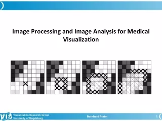
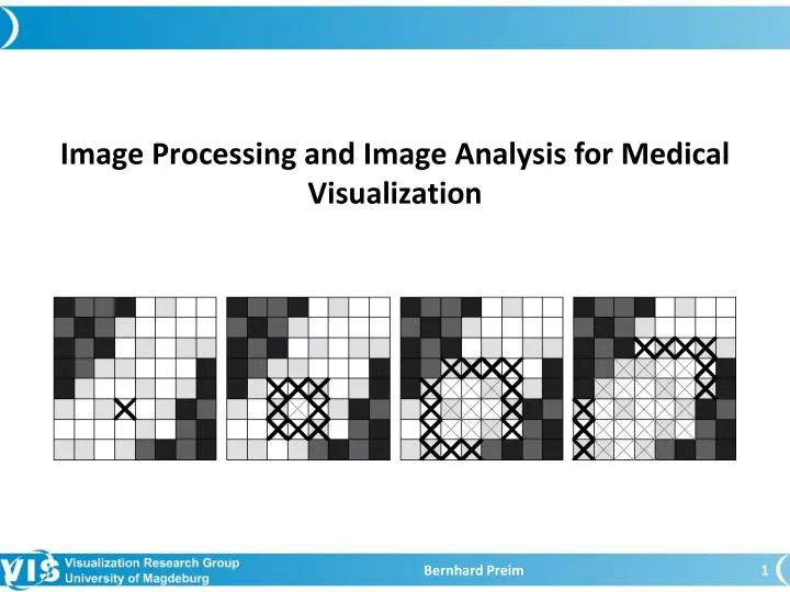
1. Image Processing and Image Analysis for Medical Visualization Bernhard Preim

2. Classification • Preprocessing • Segmentation procedures • Semi-automatic procedures • Automatic procedures • Applications: Segmentation of organs, lesions and vessels • Postprocessing with morphologic operators • Skeletization • Quantitative analysis of medical image data Bernhard Preim

3. Introduction Bernhard Preim

4. Preprocessing • Application of local or global image processing filters that support the subsequent processing • Examples: • noise reduction • edge enhancement • contrast enhancement • reduction of MR inhomogeneities Bernhard Preim

5. Preprocessing: Definitions • Histogram: Function that indicates the frequency of each grey value. • h(g) = |{p є (MN) with f(p) = g}|, ∑h(g) = M * N • Tri-modal histogram (histogram with three distinctive maxima) Bernhard Preim

6. Preprocessing: Definitions • Point-oriented operations • The values of a voxel are changed (isolated), e.g. thresholding, subtraction, lookup table • Local filters (mask, cores) • The values of a voxel are changed dependent on the values in the neighborhood. • static and dynamic filters • Problem: treatment of edges • Global operations • Histogram equalization Bernhard Preim

7. Noise Reduction Overview over the filters: • Average filter • Linear noise filter, which flattens edges • Median filter • Edge-preserving noise filter, non-linear, rank filter • Gaussian filter • Non-linear noise filter, which flattens edges • Sigma filter • Non-linear noise filter The filters (except Median) are normalized such that the sum of the absolute values is 1. Bernhard Preim

8. Noise Reduction: Median Filtering • Procedure: The sequence of the grey values is identified in a local surrounding (3x3, 5x5). • Each grey value is replaced by the value which appears in the middle during the sorting • Example: 3x3 size, value 17, surrounding: (8,12, 12, 17, 19, 19, 21, 22, 24): replace 17 by 19 • Similar filters: Minimum/maximum filter (after sorting the current pixel is replaced by the minimum/maximum value → enlargement of details) Bernhard Preim

9. Noise Reduction: Median Filtering Application of a 5x5 Median filter to an axial slice of CT data Bernhard Preim

10. Noise Reduction: Median Filtering Characteristics: • Good suppression of pulsed noise (outliers) • The average grey value of the image may vary • Edge transitions are preserved • Thin lines are suppressed Suppression of thin lines is avoidable through a special kernel form. Bernhard Preim

11. Noise Reduction: Gaussian Filter • Filtering with a discretized Gaussian function (Gaussian bell curve, weighted mean value) • Values correspond to binomial coefficients 1/16 * 1/256 * Bernhard Preim

12. Noise Reduction: Gaussian Filter Characteristics: • Noise in a small surrounding is suppressed. • Sharp edges are smoothed. Bernhard Preim

13. Noise Reduction: Gaussian Filter Gaussian filter for an MRI data set; screenshots: Vtk Reference: Schroeder et al. (1998) Bernhard Preim

14. Noise Reduction: Gaussian Filter 3D ultrasound. Left: unfiltered, middle, right: moderate and strong Gaussian filter, respectively. (Sakas, 1995) Bernhard Preim

15. Noise Feduction: Model Assumptions • Gaussian filtering assumes a normally distributed noise • CT and X-ray images: assumption holds true • MRI data: asymmetric Rician distribution CT data; Gaussian mixture model, Rician distribution (Source: Hennemuth, 2012) Bernhard Preim

16. Noise Reduction: Sigma Filter Idea: Limit the noise filtering to pixels (voxels) that do not deviate too strong from the average value. Use of a parameter sigma, which doesn not concretize “too strong”. • Calculation of the standard deviationstd_dev within a kernel. For each pixel (voxel) with p in the kernel with p(i) in [-sigma *std_dev, sigma *std_dev] calculate the average value avg For each pixel (voxel) with p in the kernel with p(i) in [-sigma *std_dev, sigma *std_dev] p(i) avg. Bernhard Preim

17. Noise Reduction: Sigma Filter Left: original CT layer, right: Sigma filtered (11x11, sigma = 1.0) (Screenshot: MeVis ILab4, data set: Uni Essen) Bernhard Preim

18. Noise Reduction: Sigma Filter Left: original CT layer, right: Sigma filtered (11x11, sigma = 1.0) (Screenshot: MeVis ILab4, data set: Uni Essen) Bernhard Preim

19. Noise Reduction: Diffusion Filtering • Diffusion filtering yields better results (edge-preserving anisotropic filtering) Reference: Lamecker at al. (2002) Bernhard Preim

20. Noise Reduction: Diffusion Filtering • Parameters primarily adjust a trade-off between accuracy (small step size, high number of iterations) and speed Bernhard Preim

21. Noise Reduction: Diffusion Filtering Original Median 5x5 Diffusion filter Bernhard Preim Bernhard Preim 22

22. Noise Reduction: Summary • Optimum quality (feature preservation and reduction of noise) is achieved with expensive diffusion filters (numerical solution of a set of partial differential equations) • Simple filters, such as Gaussian, have a higher performance. • Suitability of a filter depends on the characteristics of the noise (probability density function) Bernhard Preim

23. Reduction of MR Inhomogeneities • Fields of the coils inhomogeneous • Consequence: brightening at edges; other form of inhomogeneity: streak artifacts • Correction: via modeling (bias field) Bernhard Preim

24. Reduction of MR Inhomogeneities Correction of inhomogeneities with N3 algorithm (Sled, 1998). Screenshot: A. Schenk, MeVis Bernhard Preim

25. Preprocessing: Contrast Enhancement • Goal: higher contrasts at object edges • Idea: Difference between the image and the Laplace-filtered image (Screenshots: vtk) Bernhard Preim

26. Preprocessing: Sharpen Characteristics: • Sum of all entries: 1 • Contrast enhancement through negative values for surrounding pixels • Examples: Sharpness factor 0.5, radius 1 and 1.5, resp. Bernhard Preim

27. Preprocessing: Sharpen Application of a Sharpen filter with 11x11 kernel Bernhard Preim

28. Preprocessing: Sharpen Unsharp masking: • Idea: The strongly smoothed original image (generated e.g. through Gaussian filtering) is digitally subtracted from the original image. Thus, the unsharp areas are faded out (masked). 5x5 Gaussian filter, CT data set Uni Essen Bernhard Preim

29. Preprocessing: Problems • Contrast enhancement is combined with noise enhancement. • Noise reduction also decreases contrasts. Bernhard Preim

30. Preprocessing: Adaptive Neighborhoods • Problems during preprocessing are related to the fixed kernel sizes. In some image parts, they are too small, in others they are too large. • Idea: Adaptive neighborhoods, which adapt in size and form to local image characteristics (grey values, gradients, textures, …). • Procedure: Starting from each central pixel/voxel, pixels/voxels in the neighborhood, which are “similar” in relation to the chosen image characteristics, are searched. Bernhard Preim

31. Preprocessing: Adaptive Neighborhoods • Similarity is defined through an additive or multiplicative tolerance criterion. (i,j) is the central pixel/voxel. “f” are, e.g., grey values. “T1, T2” are threshold values. • Additive: |f(k,l) – f(i,j)|  T1 • Multiplicative: (|f(k,l) – f(i,j)| )/ f(i,j)  T2 Specific procedure: Search for pixels/voxels in the direct neighborhood that fulfill the similarity criterion. Search for all of these pixels/voxels in their neighborhood (recursive). Criterion for cancellation: no further pixels/voxels fulfill the criterion. Bernhard Preim

32. Preprocessing: Adaptive Neighborhoods Applications: • Noise suppression (Gaussian, Median) • Edges are better preserved. • Tolerance criterion depends on the type of noise. • Unsuitable in case of pulsed noise. • Histogram modification • Instead of global equalization: application in adaptive neighborhood. • Application in case of image inhomogeneities, e.g. MR data. • Contrast enhancement • Medium contrasts may be specifically enhanced through the use of adaptive neighborhoods. (Strong contrasts need no enhancement, weak contrasts can mostly be traced back to noise.) Bernhard Preim

33. Preprocessing: Highlighting of Elongated Structures Elongated structures are identified via an Eigenvalue analysis of the Hessian matrix (approximated 2nd derivatives). Major application: vasc. Structures -> vesselness filtering More about this topic: In the exercises! Bernhard Preim