Download
1 / 37
380 likes | 387 Vues
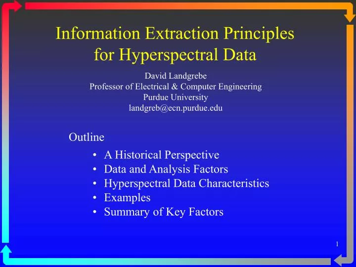
Outline. A Historical Perspective Data and Analysis Factors Hyperspectral Data Characteristics Examples Summary of Key Factors. David Landgrebe Professor of Electrical & Computer Engineering Purdue University landgreb@ecn.purdue.edu.

E N D
Outline • A Historical Perspective • Data and Analysis Factors • Hyperspectral Data Characteristics • Examples • Summary of Key Factors David Landgrebe Professor of Electrical & Computer Engineering Purdue University landgreb@ecn.purdue.edu Information Extraction Principles for Hyperspectral Data
Brief History REMOTE SENSING OF THE EARTH Atmosphere - Oceans - Land 1957 - Sputnik 1958 - National Space Act - NASA formed 1960 - TIROS I 1960 - 1980 Some 40 Earth Observational Satellites Flown
Enlarged 10 Times Image Pixels Thematic Mapper Image
6-bit data MSS 1968 8-bit data TM 1975 10-bit data Hyperspectral 1986 Three Generations of Sensors
Ephemeris, Calibration, etc. On-Board Processing Sensor Data Analysis Information Utilization Preprocessing Human Participation with Ancillary Data Systems View
Sample ImageSpace SpectralSpace Feature Space • Image Space - Geographic Orientation Data Representations • Spectral Space - Relate to Physical Basis for Response • Feature Space - For Use in Pattern Analysis
BHATTACHARYYA DISTANCE Mean Difference Term Covariance Term
Vegetation in Spectral Space Laboratory Data: Two classes of vegetation
Hughes Effect G.F. Hughes, "On the mean accuracy of statistical pattern recognizers," IEEE Trans. Inform. Theory., Vol IT-14, pp. 55-63, 1968.
Quadratic Form • Fisher Linear Discriminant - Common class covariance • Minimum Distance to Means - Ignores second moment Classifiers of Varying Complexity
Correlation Classifier • Spectral Angle Mapper • Matched Filter - Constrained Energy Minimization Classifier Complexity - con’t • Other types - “Nonparametric” • Parzen Window Estimators • Fuzzy Set - based • Neural Network implementations • K Nearest Neighbor - K-NN • etc.
Class 1 Class 2 Class 3 Class 4 Class 5 b b b b b a b a b a b a b a b a a b a a b a a b a a b a a b a a a b a a a b a a a b a a a b a a a b a a a a b a a a a b a a a a b a a a a b a a a a b a a a a a b a a a a a b a a a a a b a a a a a b a a a a a b Covariance Coefficients to be Estimated • Assume a 5 class problem in 6 dimensions Common Covar. d c d c c d c c c d c c c c d c c c c c d • Normal maximum likelihood - estimate coefficients a and b • Ignore correlation between bands - estimate coefficients b • Assume common covariance - estimate coefficients c and d • Ignore correlation between bands - estimate coefficients d
Number of Coefficients to be Estimated • Assume 5 classes and p features
Intuition and Higher Dimensional Space Borsuk’s Conjecture: If you break a stick in two, both pieces are shorter than the original. Keller’s Conjecture: It is possible to use cubes (hypercubes) of equal size to fill an n-dimensional space, leaving no overlaps nor underlaps. Counter-examples to both have been found for higher dimensional spaces. Science, Vol. 259, 1 Jan 1993, pp 26-27
The Volume of a Hypercube concentrates in the corners The Volume of a Hypersphere concentrates in the outer shell The Geometry of High Dimensional Space
Some Implications • High dimensional space is mostly empty. Data in high dimensional space is mostly in a lower dimensional structure. • Normally distributed data will have a tendency to concentrate in the tails; Uniformly distributed data will concentrate in the corners.
Volume of a hypersphere = Differential Volume at r = How can that be?
The Probability Mass at r = How can that be? (continued)
MORE ON GEOMETRY • The diagonals in high dimensional spaces become nearly orthogonal to all coordinate axes Implication: The projection of any cluster onto any diagonal, e.g., by averaging features could destroy information
STILL MORE GEOMETRY • The number of labeled samples needed for supervised classification increases rapidly with dimensionality In a specific instance, it has been shown that the samples required for a linear classifier increases linearly, as the square for a quadratic classifier. It has been estimated that the number increases exponentially for a non-parametric classifier. • For most high dimensional data sets, lower dimensional linear projections tend to be normal or a combination of normals.
A HYPERSPECTRAL DATA ANALYSIS SCHEME 200 Dimensional Data Class Conditional Feature Extraction Feature Selection Classifier/Analyzer Class-Specific Information
Finding Optimal Feature Subspaces • Feature Selection (FS) • Discriminant Analysis Feature Extraction (DAFE) • Decision Boundary Feature Extraction (DBFE) • Projection Pursuit (PP) Available in MultiSpec via WWW at: http://dynamo.ecn.purdue.edu/~biehl/MultiSpec/ Additional documentation via WWW at: http://dynamo.ecn.purdue.edu/~landgreb/publications.html .
Hyperspectral Image of DC Mall HYDICE Airborne System 1208 Scan Lines, 307 Pixels/Scan Line 210 Spectral Bands in 0.4-2.4 µm Region 155 Megabytes of Data (Not yet Geometrically Corrected)
Define Desired Classes Training areas designated by polygons outlined in white
Thematic Map of DC Mall Legend Operation CPU Time (sec.) Analyst Time Display Image 18 Define Classes < 20 min. Feature Extraction 12 Reformat 67 Initial Classification 34 Inspect and Mod. Training ≈ 5 min. Final Classification 33 Total 164 sec = 2.7 min. ≈ 25 min. Roofs Streets Grass Trees Paths Water Shadows (No preprocessing involved)
Hyperspectral Potential - Simply Stated • Assume 10 bit data in a 100 dimensional space. • That is (1024)100 ≈ 10300 discrete locations Even for a data set of 106 pixels, the probability of any two pixels lying in the same discrete location is vanishingly small.
Ephemeris, Calibration, etc. On-Board Processing Sensor Data Analysis Information Utilization Preprocessing Human Participation with Ancillary Data Summary - Limiting Factors • Scene - The most complex and dynamic part • Sensor - Also not under analyst’s control • Processing System - Analyst’s choices
Limiting Factors Scene - Varies from hour to hour and sq. km to sq. km Sensor - Spatial Resolution, Spectral bands, S/N Processing System - - Informational Value, - Separable, • Classes to be labeled - Exhaustive, • Number of samples to define the classes • Features to be used • Complexity of the Classifier
Image Space Spectral Space Feature Space Source of Ancillary Input Possibilities . - From the Ground • Ground Observations - Of the Ground • “Imaging Spectroscopy” • Previously Gather Spectra • “End Members”
Use of Ancillary Input A Key Point: • Ancillary input is used to label training samples. • Training samples are then used to compute class quantitative descriptions Result: • This reduces or eliminates the need for many types of preprocessing by normalizing out the difference between class descriptions and the data