Download
1 / 16
160 likes | 303 Vues
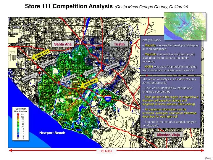
Store 111 Competition Analysis (Costa Mesa Orange County, California). Analytic Tools MapInfo was used to develop and display all map databases MapCalc was used to analyze the grid level data and to execute the spatial modeling

E N D
Store 111 Competition Analysis (Costa Mesa Orange County, California) • Analytic Tools • MapInfo was used to develop and display all map databases • MapCalc was used to analyze the grid level data and to execute the spatial modeling • KXEN was used for predictive modeling and competition analysis (www.kxen.com) Santa Ana Tustin Branch 111 Competitor 1 Competitor 5 Competitor 4 Competitor 2 Competitor 3 • The region of analysis is divided into 20 x 20 meter grid cells • Each cell is identified by latitude and longitude coordinates • Each person in the region is mapped to a discrete cell based on latitude and longitude of home address (Geo-coding) • All customer information can be summed, averaged, counted or otherwise described for each grid cell • The cell is the unit of all spatial analysis for MapCalc Main Store Newport Beach Ocean Mission Viejo 28 Miles (Berry)
Travel-Time from Store 111 (Travelshed) Ocean (Berry)
Travel-Time from Competitor Store 1 (Travelshed) Ocean (Berry)
Travel-Time from Competitor Store 2 (Travelshed) Ocean (Berry)
Travel-Time from Competitor Store 3 (Travelshed) Ocean (Berry)
Travel-Time from Competitor Store 4 (Travelshed) Ocean (Berry)
Travel-Time from Competitor Store 5 (Travelshed) Ocean (Berry)
Travel-Time All Stores (Travelsheds) Ocean Ocean Ocean Ocean Ocean Ocean Travel-Time maps from several stores treating highway travel as four times faster than city streets. Blue tones indicate locations that are close to a store (estimated twelve minute drive or less). Customer data can be appended with travel-time distances and analyzed for spatial relationships in sales and demographic factors. Ocean (Berry)
Travel-Time Surfaces for Store #111 and Competitor #4 Blue tones indicate locations that are close to a store (estimated twelve minute drive or less). The green through red tones form a bowl-like surface with larger travel-time values identifying locations that are farther away. The value stored at each grid location specify how far away it is from the store—location 103, 86 is 5 minutes away from Store #111 and 3.0 minutes away from Competitor #1. Col = 103 Row = 86 100.5 * .0 5 = 5.0 minutes From Store #111 60.8 * .0 5 = 3.0 minutes From Competitor #4 3D surface view 2D map view (Berry)
Competition Map for Store #111 and Competitor #4 The travel-time surfaces for two stores can be compared to identify the relative access advantages throughout the project area. When the two surfaces are subtracted, zero values indicate areas that require the same travel-time to both stores—equidistant (effective travel-time distance). This Combat Zone is identified where differences are small (yellow tones); positive differences indicate increasingly favorable travel-time to the Store (green tones); and negative differences indicate increasingly favorable travel-time to the Competitor (red tones). Col= 103 Row= 86 3.0 – 5.0 = -2.0 minutes (Competitor advantage) 60.8 * .0 5 = 3.0 minutes From Competitor #4 Equidistant Bisector S#111 C#4 100.5 * .0 5 = 5.0 minutes From Store #111 Ocean …note the radical difference between the simple distance solution and the combat zone solution responding to travel-time affects of the road network (Berry)
Competition Map (S#111 and C#1) Travel-Time Equidistant Bisector Equidistant Bisector Ocean Combat111_Competitor1 Competition Maps for Store #111 to its Competitors Yellow tones indicate locations that have similar travel-times to both stores (Combat Zone). Green tones identify locations where the store has a competitive advantage with darker green areas having increasing advantage. Red tones indicate areas where the competitor has an advantage. Ocean Combat111_Competitor2 Ocean Combat111_Competitor3 Combat111_Competitor3 Combat111_Competitor3 Ocean Ocean Ocean (Berry)
S#111 C#1 C#5 C#4 C#2 C#3 S#119 Ocean Customer Locations Increasing number of customers per cell (Berry)
S#111 C#1 C#5 C#4 C#2 C#3 S#119 Ocean Customer Density Surface Increasing number of customers within 1km (Berry)
Average= 287 + StDev= 581 Break point= 868 S#111 C#1 C#5 C#4 C#2 C#3 S#119 High Customer Density (Pockets) Unusually High Customer Density: Pockets of Customers Increasing number of customers within 1km Ocean (Berry)
Combat Zones (Store #111 vs. Competitor #4) Combat Zones (Berry)
Average= 287 + StDev= 581 Break point= 868 Store #111 Advantage S#111 C#1 C#5 C#4 Competitor #4 Advantage C#2 C#3 S#119 High Customer Density (Divided Pockets) Unusually High Customer Density: Competitor #4 has advantage to more pockets Increasing number of customers within 1km Ocean (Berry)