Download

1 / 12
130 likes | 251 Vues
Speed-Flow & Flow-Delay Models. Marwan AL-Azzawi. Project Goals. To develop mathematical functions to improve traffic assignment To simulate the effects of congestion build-up and decline in road networks To develop the functions to cover different traffic scenarios. Background.

E N D
Speed-Flow & Flow-Delay Models Marwan AL-Azzawi
Project Goals • To develop mathematical functions to improve traffic assignment • To simulate the effects of congestion build-up and decline in road networks • To develop the functions to cover different traffic scenarios
Background • In capacity restraint traffic assignment, a proper allocation of speed-flow in highways, plays an important part in estimating the effects of congestion on travel times and consequently on route choice. • Speeds normally estimated as function of highway type and traffic volumes, but in many instances the road geometric design and its layout are omitted. • This raises a problem with regards to taking into account the different designs and characteristics of different roads.
Speed-Estimating Models • Generally developed from large databases containing vehicle speeds on road sections with different geometric characteristics, and under different flow levels. • Multiple regression or multiple variant analysis used. • Example: S = DS – 0.10B – 0.28H – 0.006V – 0.027V* ....... (1) • DS = constant term (km/h) B = road bendiness (degrees/km) • H = road hilliness (m/km) V or V* = flow < or > 1200 (veh/h) • DS is “desired speed” - the average speed drivers would drive on a straight and level road section with no traffic flow (road geometry is the only thing restricting the speed of vehicles). • “Desired” and “free-flow” speed different - latter is speed under zero traffic, regardless of road geometry. In fact, “desired speed” is only a particular case of “free-flow speed”.
Equation of S-F Relationship • S1(V) = A1 – B1V V < F ........................ (2) • S2(V) = A2 – B2V F < V < C ............ (3) • A1 = S0 B1 = (S0 – SF) / F • A2 = SF + {F(SF – SC)/(C – F)} B2 = (SF – SC) / (C – F) • S1(V) and S2(V) = speed (km/h) • V = flow per standard lane (veh/h) • F = flow at ‘knee’ per standard lane (veh/h) • C = flow at capacity per standard lane (veh/h) • S0 = free-flow speed (km/h) • SF = speed at ‘knee’ (km/h) • SC = speed at capacity (km/h)
Flow-Delay Curves • Exponential function appropriate to represent effects of congestion on travel times. • At low traffic, an increase in flows would induce small increase in delay. • At flows close to capacity, the same increase would induce a much greater increase in delays.
Equation of F-D Curve • t(V) = t0 + aVn V < C ........................ (4) • t(V) = travel time on link t0 = travel time on link at free flow • a = parameter (function of capacity C with power n) • n = power parameter input explicitly V = flow on link • Parameter n adjusts shape of curve according to link type. (e.g. urban roads, rural roads, semi-rural, etc.) • Must apply appropriate values of n when modelling links of critical importance.
Converting S-F into F-D • If time is t = L / S equations 2 and 3 could be written: • t1(V) = L / (A1 – B1V) V < F .......................... (5) • t2(V) = L / (A2 – B2V) F < V < C ............. (6) • These equations represent 2 hyperbolic (time-flow) curves of a shape as shown in figure 3. • Use ‘similar areas’ method to calculate equations. Tables 1 in paper gives various examples of results.
Incorporating Geometric Layouts • Example - consider rural all-purpose 4 lane road. If the speed model is: S = DS – aB – bH – cV - dV* • Let: So* = DS – aB – bH. Also, if only the region of low traffic flows is taken (road geometry only affects speed at low traffic levels) then d = 0 • Hence equation is: S = S0* – cV • Constant term S0* is ‘geometry constrained free-flow speed’, and equation is geometry-adjusted speed-flow relationship. New parameter n* from equation 9 (in paper) replacing S0 by S0*. • Example - DS = 108 km/h, B = 50 degrees/km, H = 20 m/km. Then S0 = 108 – 0.10*0.5 – 0.28*20 = 97 km/h (i.e. the “free-flow” speed S0 equal to 108 km/h is reduced by 11 km/h due to road geometry).
Conclusions • New S-F models should improve traffic assignment • New F-D curves help simulate affects of congestion • Further work on-going to develop model parameters for other road types