Download
1 / 45
730 likes | 1.74k Vues
Some analytical models of nonlinear physical systems. P. 2. l. x. A. 1. k 2. l. g. k 1. O. y. Discrete Dynamical Systems : Inverted Double Pendulum : Consider the double pendulum shown:. Inverted Double Pendulum – E quation of motion.

E N D
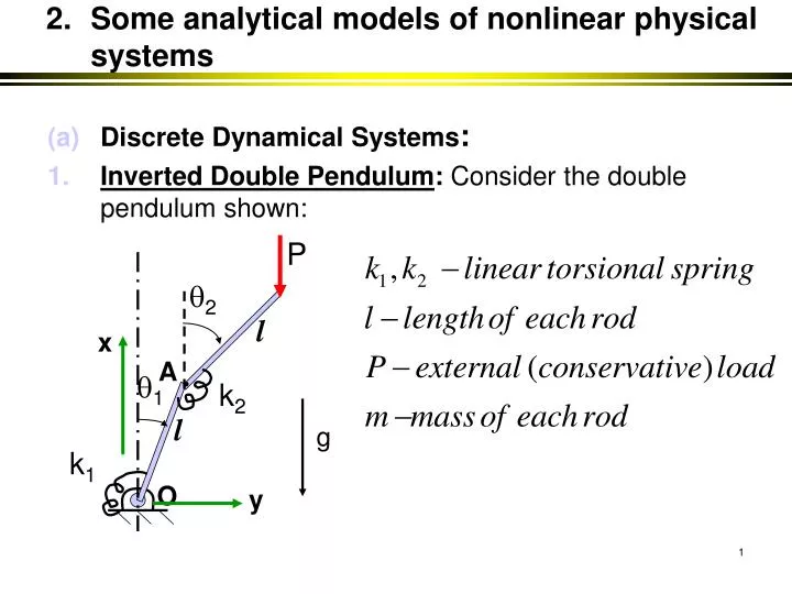
Some analytical models of nonlinear physical systems P 2 l x A 1 k2 l g k1 O y • Discrete Dynamical Systems: • Inverted Double Pendulum: Consider the double pendulum shown:
Inverted Double Pendulum –Equation of motion The equations of motion can be determined by using Lagrange’s equations: Here, • - are the generalized coordinates, • T and V- are the respective kineticand potentialEnergies for the system, • -- the generalized forces due to non-conservative effects.
Inverted Double Pendulum – Equations of motion For the double pendulum- kinetic energy:
Inverted Double Pendulum – Equations of motion Potential energy: The work done by the external force P in a virtual displacement from straight vertical position is:
Inverted Double Pendulum – Equations of motion: Equation for 1:
Inverted Double Pendulum – Equations of motion: Equation for 2:
Inverted Double Pendulum –Equations of motion: We now consider a simplified version with k1= k2=k Let Then, the equations are: Equation for 1: Equation for 2:
P 2 B l x A 1 k2 l g k1 O y Discrete dynamical systems……. 2. Inverted Double Pendulum with Follower Force: Consider the same system as in last example, except that the force P changes direction depending on the orientation of the body on which it acts. The force P now acts at an angle to the rod AB and always maintains this direction relative to the rod regardless of the position in space of the system during its oscillations.
Inverted Double Pendulum with Follower….– Equations of motion Note that the only change is in the effect of the external force P. The potential and kinetic energy expressions remain the same. So, potential energy: The work done by the external force P in a virtual displacement from straight vertical position is:
Inverted Double Pendulum with Follower– Equations of motion The virtual displacement is: The resulting equations of motion are: Thus, the generalized forces are:
Inverted Double Pendulum with Follower– Equations of motion and In the reduced case, with equal springs etc., the equations are:
ball mg g Y(t) table ground Discrete dynamical systems……. 3. Dynamics of a Bouncing Ball: Consider a ball bouncing above a horizontal table. The table oscillates vertically in a specified manner (here we assume harmonic oscillations). The motion of the ball, during free flight, is governed by Integrating once gives:
ball mg g Y(t) table ground Dynamics of a Bouncing Ball ……. Integrating once gives: Integrating again, we get: The position of the ball has to remain above the table Finally, we have the law of interaction between the table and the ball:
ball mg g Y(t) table ground Dynamics of a Bouncing Ball ……. Thus, we have the relation: These relations provide a complete description of motion of the ball. Note that, given an initial condition, we have to piece together the motion in forward time
ball mg g Y(t) table ground Dynamics of a Bouncing Ball ……. Let us now proceed in a systematic manner. For nonlinear analysis, it is always advisable to non- dimensionalize equations: So we define
ball g Y(t) mg table ground Dynamics of a Bouncing Ball ……. Ball motion: z(t)= (22g/2)Z(), Now, Integrating,
ball mg g Y(t) table ground Dynamics of a Bouncing Ball ……. Thus, we have Ball motion: Table motion: Initially: ball starts at time 0 when it is in contact with the table, and just about to leave
ball mg g Y(t) table ground Dynamics of a Bouncing Ball ……. Ball velocity at =0: Next collision at time 1 > 0 when Now, Using (3)-(5)
ball mg g Y(t) table ground Dynamics of a Bouncing Ball ……. Then, the time instant 1 is defined by (this is a relation in W’0, 1 and 0, and it depends on )
ball mg g Y(t) table ground Dynamics of a Bouncing Ball ……. When just about to contact at this time instant 1 the relative velocity is : or: On impact, the ball relative velocity changes:
ball mg g Y(t) table ground Dynamics of a Bouncing Ball ……. One can write the equations now in a more compact form: and Knowing (I,W’i), equations (A) and (B) can be used to compute (I+1,W’i+1), thus generating the trajectory.
r cooling R α heating (b) Continuous Dynamical Systems • Rotating Thermosyphon: Consider a closed circular tube in a vertical plane. The tube is filled with a liquid of constant properties, except for variation of its density with temperature in buoyancy and centrifugal terms, i.e. in body forces. One part of the loop is heated, and the other cooled. The tube is spun about the vertical axis.
r cooling R α heating Rotating Thermosyphon… There are many ways to develop a model for the system. If the tube radius ‘r’ is much smaller than the torus radius ‘R’, one can assume that there is negligible flow in the radial direction. Another approach is to average the velocity and temperature over the tube radius. Then, the equations for fluid motion are:
r cooling R α heating Rotating thermosyphon: equations… Continuity: Here, V – average flow velocity at any section ; - density of the fluid and (V) is independent of .Momentum: Here, p – fluid pressure at a section, w- shear stress at the wall
r cooling R α heating Rotating thermosyphon:Equations… Energy: where Cp- specific heat of the fluid, T – mean fluid temperature at a section, k – thermal conductivity, q’ – applied heat source per unit length. Remark: Here viscous dissipation term is neglected
r cooling R α heating Rotating thermosyphon: Equations… Simplification and nondimensionalization: Integrating the momentum eqn. (2) along the loop Shear stress: Friction factor:
Rotating thermosyphon: Equations… Simplification: Introduce the variation of density with temperature in buoyancy and centrifugal terms, and use periodicity of variables (eqn. (4)) where -kinematic viscosity, Tr-reference temperature - coefficient of thermal expansion
Rotating thermosyphon: Equations… Non-dimensional variables:
Rotating thermosyphon: Equations… Non-dimensional equations: The resulting momentum and energy equations are: Note: - combination of geometric parameter and the Prandtl number Pr. Pr > 1 for ordinary fluids (air, water etc.) and <1 for liquid metals.
Rotating thermosyphon: equations… Solution approach: The solutions to (7) and (8) can be expressed as: where as, the externally imposed heat flux can be represented in a Fourier series as: Substituting (9) and (10) in equations (7) and (8), and collecting the appropriate Fourier coefficients gives an infinite set of ordinary differential equations In the unknowns U(), Bn(), and Cn().
Rotating thermosyphon: equations… Solution approach…: It turns out that only five of these equations are independent-masterequations. The remaining equations are linear equations for the remaining variable (called “slave variables” and “slave equations”). Equation (8) gives:
Rotating thermosyphon: equations… Solution approach…: Collecting terms of different n’s give:
Rotating thermosyphon: Equations… Solution approach…: Now, considering equation (7) we get: Evaluating the two integral terms on the right-hand side, it is clear that only coefficients of will survive. Thus, we get Equations (11) and (12) govern the dynamics.
V X (b) Continuous Dynamical Systems 2. Buckling of Elastic Columns: Consider a thin beam that is initially straight. O xyz is coordinate system with x-y plane coinciding with undisturbed neutral axis of the beam. Let EI is the bending stiffness
V X Buckling of elastic….. V(s) – vertical displacement of the centroidal axis, X – distance measured along the centroidal axis from left end. Define: Then, the strain energy of the system is:
y, v z, w a x, u (b) Continuous Dynamical Systems 3. Thin rectangular plates: Consider a thin plate that is initially flat. Oxyz is coordinate system with x-y plane coinciding with undisturbed middle surface of the plate. Let h – plate thickness. The equations of motion for the plate, for moderately large displacements – von Karmanequations. In here, we give a short review of the derivation of these equations.
Ny F z Nxy Nx Nx Nxy x Ny y Thin rectangular plates….. Consider a differential plate element: The equations in the three directions are:
Ny F z Nxy Nx Nx Nxy x Ny y Thin rectangular plates….. The constitutive equations for a linearly elastic and isotropic material are: In these expressions, N, Ni – forces, M - moments
Ny F z Nxy Nx Nx Nxy x Ny y Thin rectangular plates….. The constitutive equations for a linearly elastic and isotropic material are: Also u,v,w – displacements Substituting the force – displacement relations in the dynamic equations give:
Thin rectangular plates….. The dynamic equations for a plate made of linearly elastic and isotropic material are then simplified by introducing a stress function such that: Then, (1) and (2) are automatically satisfied if in- plane inertia terms are neglected. Furthermore, the expressions (7)-(9) can be substituted in (3) to get equation for transverse displacement. Also, a compatibility condition is (gives an equation for ):
2 b 1 a (b) Continuous Dynamical Systems 4. Flow between concentric rotating cylinders: Consider two concentric cylinders with radii a, b; Let 1, 2 – angular velocities of inner and outer cylinders; let (ur,uθ,uz) – velocity components in a cylindrical coordinate system; p – pressure at a point; We now define the equations of motion for the system.
2 b 1 a Flow between concentric rotating…. Equations of motion for the system: In cylindrical coordinate system the NS equations are
2 b 1 a Flow between concentric rotating…. Equations of motion for the system: and There is also the equation for mass conservation: The basic flow is defined by:
2 b 1 a Flow between concentric rotating…. The basic flow…: Equations (3) have solution of the form Let us consider perturbations to the basic flow: We can then obtain linearized equations about the basic flow.
Flow between concentric rotating…. Linearized equations about the basic flow: