Download

1 / 65
650 likes | 738 Vues
Session 5a. Overview. Portfolio Optimization Parametric Approach Array Functions Scenario Approach Put Options Shorting. 4 Basic Matrix Operations. Sum Product Transpose Matrix Multiplication Inverting Matrices. Sum Product.

E N D
Overview Portfolio Optimization • Parametric Approach • Array Functions • Scenario Approach • Put Options • Shorting Decision Models -- Prof. Juran
4 Basic Matrix Operations • Sum Product • Transpose • Matrix Multiplication • Inverting Matrices Decision Models -- Prof. Juran
Sum Product Decision Models -- Prof. Juran
Notes: r = i and c = j. In other words, the two matrices must have the same number of rows as each other and the same number of columns as each other. They do not need to be square matrices (where r = c and i = j). Decision Models -- Prof. Juran
A B C D 1 7 4 6 2 5 2 11 3 4 9 3 8 5 10 12 1 6 =SUMPRODUCT(A1:C2,A4:C5) 7 208 8 Decision Models -- Prof. Juran
Transpose For matrix A, Decision Models -- Prof. Juran
Notes: • If A is an r x c matrix, then must be a c x r matrix. • A does not need to be a square matrix. Decision Models -- Prof. Juran
There is an Excel function for this purpose, called TRANSPOSE. This function is one of a special class of functions called array functions. In contrast with most other Excel functions, array functions have two important differences: • They are entered into ranges of cells, not single cells • You enter them by pressing Shift+Ctrl+Enter, not just Enter Decision Models -- Prof. Juran
Using the spreadsheet above as an example, we start by selecting the entire range A4:C6. Then type into the formula bar =TRANSPOSE(A1:C2) Press Shift+Ctrl+Enter, and curly brackets will appear round the formula (you can’t type them in). Decision Models -- Prof. Juran
Matrix Multiplication For matrices A and B, Decision Models -- Prof. Juran
Inverting Matrices First, define a square matrix Ij as a matrix with j rows and j columns, completely filled with zeroes, except for ones on the diagonal: This special matrix is called the identity matrix. Decision Models -- Prof. Juran
Now, for a square matrix A with j rows and j columns, there may exist a matrix called A-inverse (symbolized ) such that: Not all square matrices can be inverted, a fact that has implications for regression analysis. Decision Models -- Prof. Juran
Remember: • Select the entire range A5:B6 before typing the formula. • Press Shift+Ctrl+Enter. Decision Models -- Prof. Juran
Parametric Approach Decision Models -- Prof. Juran
Parametric Approach Decision Models -- Prof. Juran
s 2 s 2 2 s 1 2 3 Parametric Approach The means are: = 0.14, = 0.11, = 0.10. μ μ μ 1 2 3 The variances are: = 0.20, = 0.08, = 0.18. The correlations are: = 0.8, = 0.7, and = 0.9. ρ ρ ρ 12 13 23 Decision Models -- Prof. Juran
Parametric Approach (a) Determine the minimum-variance portfolio that attains an expected annual return of at least 0.12, with no shorting of stocks allowed. (b) Draw the efficient frontier for portfolios composed of these three stocks. (c)Determine the minimum-variance portfolio that attains an expected annual return of at least 0.12, with shorting of stocks allowed. Decision Models -- Prof. Juran
Managerial Problem Definition Decision Variables We need to allocate 100% of the available funds to the three stocks. Objective We want to minimize risk. Constraints The expected return on the portfolio must be at least 12% (or 0.12). All of the money must be invested. No shorting is allowed. Decision Models -- Prof. Juran
Formulation Decision Variables Define xi to be the proportion of the portfolio allocated to stock i. The decision variables are three proportions: x1, x2, and x3. Decision Models -- Prof. Juran
Formulation Decision Models -- Prof. Juran
Formulation Decision Models -- Prof. Juran
Solution Methodology Decision Models -- Prof. Juran
Solution Methodology The decision variables are in B14:D14. Cell B18 keeps track of constraint (1). Cell E14 keeps track of constraint (2). We can comply with constraint (3) by selecting “assume nonnegative” in the Solver Options box. The range H8:J10 uses the HLOOKUP Excel function to calculate the covariances. Decision Models -- Prof. Juran
Solution Methodology Cell B20 uses two of Excel’s matrix functions, MMULT and TRANSPOSE, to calculate the portfolio variance. If you use these functions, you will want to learn more about working with “arrays” in Excel, an advanced topic beyond the scope of this course. In this case, you need to know not to type in the “curly brackets”; instead, type in the rest of the function and then Ctrl+Shift+Enter. The curly brackets will appear automatically. You will get a #VALUE! Error message if you do this wrong. Decision Models -- Prof. Juran
Optimal Solution Decision Models -- Prof. Juran
Optimal Solution The least risky way to invest these three stocks while having an expected return of at least 12% is to invest 33.3% in Stock 1 and 66.7% in Stock 2. This portfolio will have an expected return of 12% and a standard deviation of return of 32.1%. Decision Models -- Prof. Juran
Parametric Approach, cont. (c)Determine the minimum-variance portfolio that attains an expected annual return of at least 0.12, with shorting of stocks allowed. All we need to do here is remove the nonnegativity constraint and re-run Solver. Decision Models -- Prof. Juran
Optimal Solution With shorting allowed, The least risky way to invest these three stocks while having an expected return of at least 12% is to sell Stock 3 short in an amount equivalent to 81.6% of the available funds, and invest 6.1% in Stock 1 and 175.4% in Stock 2. This portfolio will still have an expected return of 12%, but a standard deviation of return of only 25.7% (as opposed to 32.1% with no shorting allowed). Decision Models -- Prof. Juran
Juran’s Lazy Portfolio • Invest in Vanguard mutual funds under university retirement plan • No shorting • Max 8 mutual funds • Rebalance once per year • Tools used: • Excel Solver • Basic Stats (mean, stdev, correl, beta, crude version of CAPM) Decision Models -- Prof. Juran 36
Scenario Approach Kate Torelli, a security analyst for Lion Fund, has identified a gold mining stock (ticker symbol GMS) as a particularly attractive investment. GMS is a highly leveraged company, so it is quite a risky investment by itself. She would therefore like to hedge the stock purchase — that is, reduce the risk of an investment in GMS stock. Decision Models -- Prof. Juran
Scenario Approach Currently GMS is trading at $100 per share. Torelli has constructed seven scenarios for the price of GMS stock one month from now. Decision Models -- Prof. Juran
Hedging with Put Options Torelli called an options trader at a large investment bank for quotes. The prices for three (European-style) put options are shown. Torelli wishes to invest $10 million in GMS stock and put options. Decision Models -- Prof. Juran
Return on Investment Decision Models -- Prof. Juran
Modeling Put Options For a put option i, the return under any scenario j is given by: Where Ki is the strike price and Ci is the cost of the option. Decision Models -- Prof. Juran
Scenario Approach, cont. Decision Models -- Prof. Juran
Scenario Approach, cont. Decision Models -- Prof. Juran
Scenario Approach, cont. Decision Models -- Prof. Juran
Example Let’s say Kate buys $7 million worth of GMS stock, and $1 million worth of each put option. This means that (x1, x2, x3, x4) = (7000, 1000, 1000, 1000). Under scenario 3, her return would be Decision Models -- Prof. Juran
Example, cont. Using the same procedure, it can be shown that for this particular allocation of assets, the seven scenarios would have returns as follows: Decision Models -- Prof. Juran
7 å = m R P j j R = 1 j = + + + + + + R P R P R P R P R P R P R P 1 1 2 2 3 3 4 4 5 5 6 6 7 7 ( ) ( ) ( ) ( ) ( ) ( ) ( ) ( ) ( ) ( ) ( ) ( ) ( ) ( ) = + - + - + - + - + + 500 0 . 05 900 0 . 1 2300 0 . 2 2200 0 . 3 538 0 . 2 5670 0 . 1 11878 0 . 05 ( ) ( ) ( ) ( ) ( ) ( ) ( ) = + - + - + - + - + + 25 90 460 660 108 567 594 = - 132 Example, cont. Therefore, the expected return on this particular allocation of assets is calculated as follows: Decision Models -- Prof. Juran
( ) 7 å 2 = - m s R P j R j R = 1 j ( ) ( ) ( ) ( ) ( ) ( ) ( ) 2 2 2 2 2 2 2 = - m + - m + - m + - m + - m + - m + - m R P R P R P R P R P R P R P 1 1 2 2 3 3 4 4 5 5 6 6 7 7 R R R R R R R ( ( ) ) ( ) ( ( ) ) ( ) ( ( ) ) ( ) ( ( ) ) ( ) ( ( ) ) ( ) ( ( ) ) ( ) ( ( ) ) ( ) 2 2 2 2 2 2 2 = - - + - - - + - - - + - - - + - - - + - - + - - 500 132 0 . 05 900 132 0 . 1 2300 132 0 . 2 2200 132 0 . 3 538 132 0 . 2 5670 132 0 . 1 11878 132 0 . 05 ( ) ( ) ( ) ( ) ( ) ( ) ( ) ( ) ( ) ( ) ( ) ( ) ( ) ( ) 2 2 2 2 2 2 2 = + - + - + - + - + + 632 0 . 05 768 0 . 1 2168 0 . 2 2068 0 . 3 406 0 . 2 5802 0 . 1 12010 0 . 05 = + + + + + + 19 , 942 59 , 054 940 , 449 1 , 283 , 565 32 , 962 3 , 366 , 307 7 , 211 , 937 = 12 , 914 , 216 = 3 , 594 Example, cont. Finally, to calculate the standard deviation of the returns under this particular allocation of assets: Decision Models -- Prof. Juran