Download

1 / 28
280 likes | 298 Vues
THE MECHANICS OF DEMAND AND PRODUCTION. FIFTH LECTURE February 21, 2012. William R. Eadington, Ph.D. Professor of Economics, College of Business Director, Institute for the Study of Gambling and Commercial Gaming University of Nevada, Reno www.unr.edu/gaming.

E N D
THE MECHANICS OF DEMAND AND PRODUCTION FIFTH LECTURE February 21, 2012 William R. Eadington, Ph.D. Professor of Economics, College of Business Director, Institute for the Study of Gambling and Commercial Gaming University of Nevada, Reno www.unr.edu/gaming
POSSIBLE SESSIONS WITH THE GRADER • Times to consider: • Tuesday 4:15 to 5:15 • Thursday 4:15 to 5:15 • Thursday 7:00 to 8:00
SIMPLE CALCULUS CONCEPTS • Consider Y = f(X) = a + b*X + c*X2 In general, Y = sum of terms of form ai*Xn • A derivative is the Rate of Change of Y as X changes, written dY/dX = n*ai*Xn-1summed over all terms • dY/dX = coef*exp.*X(n-1)summed over all terms • Example: When driving a car, let D = distance traveled, and t = time from start • Suppose D = a + b*t + c*t2 • ThendD/dt = b + 2*c*t = velocity • Then d2D/dt2 = 2*c = acceleration
APPLICATIONS TO CURRENT WORK • Consider Q = a + b*P as a demand curve • TR = P*Q = a*P + b*P2 • MR = dTR/dP = a + 2*b*P • Optimization occurs when dY/dX = 0 • Inverse Demand curve: P = c + d*Q • Consider elasticity: Ƞ = percent change in Q/percent change in P = (dQ/Q)/(dP/P) = (dQ/dP)*P/Q
PROBLEM OF THE WEEK: 4-30 Japan has 4,350 miles of expressway – all toll roads. In fact, the tolls are so high that many drivers avoid using expressways. A typical 3 hour expressway trip can cost $47. A new $12 billion bridge over Tokyo Bay that takes 10 minutes and costs $25 rarely is busy. One driver prefers snaking along Tokyo’s city streets for hours to save $32 in tolls. Assume that the daily demand curve for a particular stretch of expressway is: P = 800 yen - .16 Q. a. At what price-quantity point does this demand curve have a price elasticity of one? b. Assume the government wishes to maximize its revenues from the expressway, what price should it set? And how much revenue does it generate at this price? c. Suppose that traffic engineers have determined that the efficient utilization of this particular toll road is 4,000 cars per day. This traffic level represents an optimum tradeoff between congestion (with its associated reduction in speeds and increase in accidents) between expressways and surface roads. If 4,000 cars per day is the socially efficient utilization of the toll road, what price should be set on the toll road? And how much revenue is collected by the government?
DEMAND, TOTAL REVENUE, & MARGINAL REVENUE $ 60 Elastic demand (n > 1) Ticket price (in dollars) n = 1 30 Inelastic demand (n < 1) Q $ 6,000 Total revenue (in dollars) Q 200 Quantity of Theater tickets
OTHER DEMAND INFLUENCES Complements versus substitutes Cross price elasticity of demand orȠxy = dQx/dPy*Px/Qy
CROSS PRICE ELASTICITY For substitutes, ηXY > 0 If the price of Pepsi rises, the demand for Coke rises For complements, ηXY < 0 If the price of peanut butter rises, the demand for jelly falls
INCOME ELASTICITY Income elasticity of demand Normal goods – demand rises as income increases (>0) Inferior goods – demand falls as income increases (<0) Luxury goods – demand rises more than proportionately as income increases (>1) orȠI = dQx/dI*I/Qx
NETWORK EFFECTS Demand for a good increases as the number of users of the good increases => “Winner Take All” technology? Telephone networks v. Voice-Over Internet Mail: The internet versus the postal system Microsoft Outlook versus Netscape Beta-Max versus VHS High Definition DVD versus Blu-Ray Without critical mass, a product will die FAX machines 3-D TV
PRODUCT LIFE CYCLE: Consider gaming in Reno Q Introduction Growth Maturity Decline Industry quantity of output Product life cycle T Time
DEMAND ESTIMATION Three general techniques interviews surveys, focus groups, questionnaires price experimentation track changes in sales when prices change statistical analysis Cross-section versus time series must account for omitted variables and other issues
INTERPRETING DEMAND FUNCTIONS • Mathematical representations of demand curves. • Example: • Law of demand holds (coefficient of PX is negative). • X and Y are substitutes (coefficient of PY is positive). • X is an inferior good (coefficient of M is negative).
LINEAR DEMAND FUNCTIONS AND ELASTICITIES Income Elasticity Own Price Elasticity Cross Price Elasticity General Linear Demand Function and Elasticities:
EXAMPLE OF LINEAR DEMAND • Qd = 10 - 2P. • Own-Price Elasticity: (-2)P/Q. • If P=1, Q=8 (since 10 - 2 = 8). • Own price elasticity at P=1, Q=8: (-2)(1)/8= - 0.25
LOG-LINEAR DEMAND General Log-Linear Demand Function:
EXAMPLE OF LOG-LINEAR DEMAND Qd = A*P-2 = A/P2 ln(Qd) = ln(A) - 2 ln(P) Own Price Elasticity: -2
GRAPHICAL REPRESENTATIONS OF LINEAR AND LOG-LINEAR DEMAND P Q P D D Q Linear Log Linear
REGRESSION ANALYSIS One use is for estimating demand functions Important terminology and concepts: Least Squares Regression model: Y = a + bX + e. Least Squares Regression line: Confidence Intervals t-statistic R-square or Coefficient of Determination F-statistic
EXAMPLE • Use a spreadsheet to estimate the following log-linear demand function:
INTERPRETING THE REGRESSION OUTPUT • The estimated log-linear demand function is: • ln(Qx)= 7.58 - 0.84 ln(Px) • Own price elasticity: -0.84 or 0.84 (inelastic) • How good is the estimate? • F-statistic significant at the 1 percent level • t-statistics of 5.29 and -2.80 indicate that the estimated coefficients are statistically different from zero • R-square of 0.17 indicates the ln(PX) variable explains only 17 percent of the variation in ln(Qx)
ESTIMATING DEMANDTHE IDENTIFICATION PROBLEM $ Three different equilibriums do not map out the demand curve; what do they map out? S1 S2 Price (in dollars) P1 D1 P2 D2 S3 P3 D3 Estimateddemand Q Q1 Q2 Q3 Quantity
PRODUCTION FUNCTIONS A production function specifies maximum output from given inputs: Technological efficiency: Maximum Q for given levels of x1,x2, …, xn; challenge for the production engineers
DEFINITION OF EFFICIENCY • Technological efficiency: Extracting the maximum amount of output from any given mix of inputs • Cost efficiency: Among all the technologically efficient combinations of inputs to achieve a given level of output, which can be acquired at least cost • Implications of efficiency concepts applied to agriculture: See the documentary FOOD, INC. (available as streaming video on NETFLIX)
RETURNS TO SCALE The relation between output and a proportional variation of all inputs together Increasing returns to scale - if inputs double, output more than doubles Decreasing returns to scale - if inputs double, output less than doubles Constant returns to scale- if inputs double, output doubles
RETURNS TO A FACTOR The relation between output and the variation in only one input, holding all other inputs constant Total product - amount of output, Q, obtained when an input, L, increases Average product Q/L Marginal product Q/L