Download
1 / 23
230 likes | 352 Vues
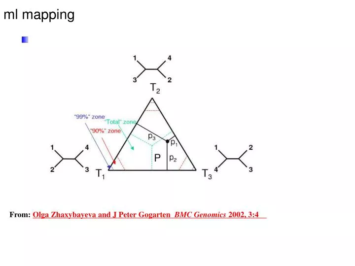
ml mapping. From: Olga Zhaxybayeva and J Peter Gogarten BMC Genomics 2002, 3:4 . L i. p i =. L 1 +L 2 +L 3. N i. p i . N total. Alternative Approaches to Estimate Posterior Probabilities. Bayesian Posterior Probability Mapping with MrBayes (Huelsenbeck and Ronquist, 2001).

E N D
ml mapping From: Olga Zhaxybayeva and J Peter Gogarten BMC Genomics 2002, 3:4
Li pi= L1+L2+L3 Ni pi Ntotal Alternative Approaches to Estimate Posterior Probabilities Bayesian Posterior Probability Mapping with MrBayes(Huelsenbeck and Ronquist, 2001) Problem: Strimmer’s formula only considers 3 trees (those that maximize the likelihood for the three topologies) Solution: Exploration of the tree space by sampling trees using a biased random walk (Implemented in MrBayes program) Trees with higher likelihoods will be sampled more often ,where Ni - number of sampled trees of topology i, i=1,2,3 Ntotal – total number of sampled trees (has to be large)
Illustration of a biased random walk Figure generated using MCRobot program (Paul Lewis, 2001)
sites versus branches You can determine omega for the whole dataset; however, usually not all sites in a sequence are under selection all the time. PAML (and other programs) allow to either determine omega for each site over the whole tree, , or determine omega for each branch for the whole sequence, . It would be great to do both, i.e., conclude codon 176 in the vacuolar ATPases was under positive selection during the evolution of modern humans – alas, a single site does not provide sufficient statistics ….
PAML – codeml – branch model dS -tree dN -tree
sites model in MrBayes The MrBayes block in a nexus file might look something like this: begin mrbayes; set autoclose=yes; lset nst=2 rates=gamma nucmodel=codon omegavar=Ny98; mcmcp samplefreq=500 printfreq=500; mcmc ngen=500000; sump burnin=50; sumt burnin=50; end;
MrBayes analyzing the *.nex.p file • The easiest is to load the file into excel (if your alignment is too long, you need to load the data into separate spreadsheets – see here execise 2 item 2 for more info) • plot LogL to determine which samples to ignore • for each codon calculate the the average probability (from the samples you do not ignore) that the codon belongs to the group of codons with omega>1. • plot this quantity using a bar graph.
the same after rescaling the y-axis plot LogL to determine which samples to ignore
copy paste formula enter formula for each codon calculate the the average probability plot row
To determine credibility interval for a parameter (here omega<1): Select values for the parameter, sampled after the burning. Copy paste to a new spreadsheet,
Sort values according to size, • Discard top and bottom 2.5% • Remainder gives 95% credibility interval.
hy-phy Results of an anaylsis using the SLAC approach more output might still be here
Hy-Phy -Hypothesis Testing using Phylogenies. Using Batchfiles or GUI Information at http://www.hyphy.org/ Selected analyses also can be performed online at http://www.datamonkey.org/
Alternatively, especially if the the two models are not nested, one can set up two different windows with the same dataset: Example testing for dN/dS in two partitions of the data –John’s dataset Model 1 Model 2
Example testing for dN/dS in two partitions of the data --John’s dataset Simulation under model 2, evalutation under model 1, calculate LR Compare real LR to distribution from simulated LR values. The result might look something like this or this
16S rRNA phylogeny colored according to tyrRS type Under the assumption that both types were present in the bacterial ancestor and explaining the observed distribution only through gene loss: 133 taxa and 58 gene loss events, 34 losses of type A, 23 of type B Green - Type A tyrRS Red - Type B tyrRS Blue - Both types of tyrRS Andam, Williams, Gogarten 2010 PNAS
LGT3State Method Simulated under "loss-only" model; likelihood under HGT model • Generated 1000 bootstrap trees under loss-only model Real data under HGT model
2 7 4 5 6 3 8 1 4 2 5 6 7 8 1 3
5 4 6 3 7 2 8 1 ori