Download
1 / 55
550 likes | 562 Vues
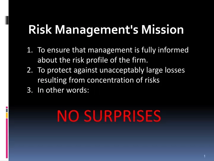
Risk Management's Mission. To ensure that management is fully informed about the risk profile of the firm. To protect against unacceptably large losses resulting from concentration of risks In other words: NO SURPRISES. How does risk management avoid surprises?.

E N D
Risk Management's Mission To ensure that management is fully informed about the risk profile of the firm. To protect against unacceptably large losses resulting from concentration of risks In other words: NO SURPRISES
How does risk management avoid surprises? • Take responsibility for accurately portraying possible outcomes • Any risk manager using the words “perfect” and “storm” in the same sentence should be fired on the spot • Three primary approaches, all of which are necessary: • Liquidity • Use markets to limit exposure • Distribution • Expressed as probabilities of gains and losses • Facilitates comparisons • Attribution • Expressed in terms specific to a given market • Facilitates action
Controlling risk [Section 6.1] • The principal tool for controlling risk should be a disciplined use of stop-loss limits • This can only as good as management discipline in taking stop-loss limits seriously – extending new capital only when the trader can make a good case for a strategy yielding results if given more time • Making sure that current position is properly marked-to-market at least daily is critical – you don’t want to be dealing with a trader who knows he’s through his stop-loss limit when you don’t • This also requires tools for managing the liquidation risk of positions that need to be closed-out because of stop-loss limits
Controlling risk • Similar issues exist for many risk management problems: • Control of trading risk through stop-loss limits and control of liquidation exposure • Control of counterparty credit risk through limits requiring settlement based on size of exposure and credit quality (e.g., downgrade provisions) and control of settlement exposure • Control of investment risk through limits on shortfall in funding of obligations (e.g., contingent immunization) and control of liquidation exposure
Controlling risk • Key principles for stop-loss limits • Careful and continuous tracking of market prices of existing positions • Sensible choices of limit size relative to trader expertise and trading strategy • Good procedures for review of requests to exceed limits • Analysis of reasons for large losses and large gains • Financing plans
Controlling risk • Key principles for liquidation risk • Recognition of the non-normal distribution of financial variables • The need for simulation • The need to consider subjective probabilities as well as objective frequencies • The distinction between diversifiable and non-diversifiable risk • The use of arbitrage theory to decompose risks • The need to consider periods of reduced liquidity • The need to distinguish degrees of illiquidity with different tools to handle each type
Why is analysis of the tails of distributions so difficult? • Any statistical analysis (financial or non-financial) that attempts to give a good representation of extremely unlikely events (tails of distributions) is particularly difficult • This is just as true of physical statistical analysis (e.g, probability of a nuclear plant accident) as it is of a financial statistical analysis (e.g., probability of a stock market crash) • The farther out your go in the tail, the fewer historical instances you have to test your theories against • Very small changes in inputs can lead to large changes in tail estimates
An example to illustrate the difficulty of tail estimation • You are trying to describe the distribution of a variable for which you have a lot of historical data that strongly supports a normal distribution with a mean of 5.00% and standard deviation of 2.00% • Suppose you suspect that there is a possibility that there will be a “regime change” that will create a very different distribution. Let’s say you guess there is a 5% chance of this distribution which you estimate as a normal distribution with a mean of 0.00% and standard deviation of 10.00% • If all you cared about was the mean of the distribution, this wouldn’t have much impact – lowering the mean from 5.00% to 4.72% • Even if you were concerned with both mean and standard deviation it wouldn’t have a huge impact – the standard deviation goes up from 2.00% to 3.18%, so the Sharpe ratio would drop from 2.50 to 1.48 • But if you were concerned with how large a loss you could have 1.00% of the time, it would be a change from a gain of 0.33% to a loss of 8.70% • This illustrates the point that when you are concerned with the tail of the distribution, you need to be very concerned with subjective probabilities and not just with objective frequencies. • When your primary concern is just the mean, or the mean and standard deviation, then your primary focus should be on choosing the most representative historical period and on objective frequencies. This might be typical for a mutual fund. • These calculations were produced with the spreadsheet “MixtureOfNormals”
Myths about reporting on distributions • Not all major firms utilize simulation • Monte Carlo simulation requires a lot of computing capacity and is expensive to develop • Monte Carlo simulation is closely tied to assumptions of normal distributions • Historical simulation exactly reproduces the “actual” distribution
VaR and Stress Tests: Lessons from the crisis[Chapter 7] • There is never any excuse for a statistical computation such as VaR to ignore fat-tailed distributions, non-linear joint distributions or non-linear payouts • Dictates the use of simulation methodology, but leaves open choices between historical and Monte Carlo simulations or blends of the two • All statistical computations such as VaR must be complemented by stress tests • To account for temporary periods of illiquidity in normally liquid markets • To account for crisis events that are not just extreme observations from the same distribution as everyday returns • Value-at-risk measures were never designed to deal with highly-complex, highly-illiquid instruments, which is where the real problems came from • All statistical computations such as VaR must properly reflect positions in less liquid instruments and illiquidity due to concentrated positions in liquid instruments • Positions that can only be represented by a liquid proxy must separately model differences between the actual product and the liquid proxy • Concentrated positions require modeling of potential cost of liquidating over a longer time period or of impact of a large position on market
Methodology for reporting on distributions • With rare exceptions, only simulation calculations should be used • For linear positions and normal distributions, Monte Carlo simulation can easily reproduce the exact same results as variance-covariance • The variance-covariance approach becomes cumbersome to use once you have either non-normal distributions or non-linear positions (such as options) • Variance-covariance can still be useful as a quick first approximation • Simulation approaches, both historical and Monte Carlo, are easy to adapt to non-normal distributions and non-linear positions • Simulation approaches can easily handle more complex questions, such as the distribution of losses from the high point to low point (which may be of particular relevance to fund managers)
Where do the position numbers come from? • Details of position reporting fit naturally with attribution reporting, so we’ll cover the topic in our next lecture • A few general points: • It’s vital that the source of position reports tie to the same data sources as official P&L reports; otherwise the firm could be seriously misled about risk • Simulation’s “one path at a time” computation lends itself easily to full representation of positions through the same models that are used to calculate official P&L • In practice, this full representation may be too inefficient in terms of running time and development time, so more concise representations may be needed (but resulting loss of accuracy should be estimated) • It will often be an issue that the full details of a contract cannot be represented in any computer system. • Senior risk managers worry more about “the risks they don’t know about” than the risks they do
Simulation Methodology All simulation is based on historical market data but not historical positions Statistical distribution of historical returns, based on historical positions, can be useful in analysis of management style (we’ll look at an example from JPMorgan’s Annual Report), but cannot fully reflect current risks (e.g., style drift) For some risk positions, such as management of exposure to hedge funds, this may be the only type of reporting available General advantages of simulation Path-by-path approach makes risk attribution and allocation easy Can use the same system for estimating distributions that you use for scenario analysis
Simulation Methodology Advantages of historical simulation Simplicity Implementation Assumptions Explanation Advantages of Monte Carlo simulation Flexibility Choose best estimation method for each parameter Choose best data set for each parameter Ease in handling missing data Ease in handling asynchronous data Ease in combining data from different sources For time periods longer than a few weeks, Monte Carlo is a necessity, due to paucity of independent historical periods For details, see Section 7.1
Stress Testing • Stress tests can be based on either hypothetical scenarios or historical replays (see section 7.2) • In either case, careful choices need to be made about the length of time during which market illiquidity is assumed • In historical replays, must make sure that values are chosen in a way that applies to all current positions , so even an historical replay is a type of hypothetical scenario • The key to development of hypothetical scenarios is specification of an economically plausible combination of systematic risk factors • Some key issues: • How to define stress tests for non-traded (i.e., illiquid) factors ? • Should scenarios be developed down to the same level of detail as VaR? • Given the small number of stress tests that can be defined by full scenarios or full historical replays, is there a computational way to produce supplementary stress tests? • Historical replays and computational approaches are inadequate without hypothetical scenarios. You need to guard against economically plausible events that have no historical precedent – e.g. the breakup of the Euro • Since the Long Term Capital Management failure, there has been a recognition of a need to create hypothetical scenarios that are portfolio specific, representing high correlations that occur not because of economic forces but due to market factors such as exit of a major competitor, forced liquidation of a portfolio, or competitors deliberately taking positions in the opposite direction of a portfolio with perceived liquidity issues.
Creating plausible but meaningful stress scenarios • It is often claimed that a large nationwide reduction in housing prices would have been rejected as an implausible stress scenario • From The Economist, 12/9/04: “Calculations by The Economist suggest that house prices have hit record levels in relation to incomes in America, Australia, Britain, France, Ireland, the Netherlands, New Zealand and Spain. In other words, ratios of prices to incomes are now above levels that have proved unsustainable in the past. Taking the average ratio of house prices to incomes in 1975-2000 as a baseline, American house prices are now almost 30% overvalued.” • This type of detailed analysis from a mainstream source indicates that implausibility was unlikely to have been the issue. • Far more likely, in my view, was the misrepresentation of CDO tranches as sufficiently liquid to allow consideration of only very short-term stress scenarios
How to define stress tests for non-traded (illiquid) factors? Different types of illiquidity require different approaches: • Positions of sporadic liquidity or illiquid size need an add-on to reflect that even after a period of general market illiquidity ends, it will still require extra time to liquidate such positions • Instruments that require a liquid proxy have a natural time frame that is longer than for standard stress tests (closer in nature to credit stress tests). We’ll discuss further in session on model risk. • Contract details that cannot be represented in the computer system require special handling • A clever approach used by JPMorgan is to incent traders to identify potential longer term losses due to unusual events (see “Risk identification for large exposures” in JPMorgan Annual Report). Traders who suffer losses from unusual events they identified in advance are treated more generously.
Level of detail for stress scenarios? An important question for hypothetical scenarios is whether to develop scenarios down to the same level of detail as VaR • Argument for is that otherwise you are ignoring components of risk • Argument against is that you if there’s no necessary relationship to systematic factors defining the scenario, you may be producing nothing but (possibly risk-offsetting) noise • I believe the best approach is to just specify the scenarios for the most important variables (systematic risk, key economic indicators, principal components) and use Monte Carlo simulation to find the “plausible” combination of less important variables that is most unfavorable to the current portfolio • Use as a starting point a full specification of the important variables with less important variables set to zero. • Use Monte Carlo to vary less important variables, assuming no correlation between less important variables. The important variables can be varied in the Monte Carlo by changing just a single variable and assuming 100% correlation between the important variables. • Consider the worst loss that has probability equal to the starting point
Computational approach to supplementary stress tests • The amount of work required to specify and understand a detailed hypothetical or historical replay scenario limits the total number of scenarios that can be considered • Possible approaches (from Barry Schachter, “How Well Can Stress Tests Complement VaR?”): • Worst Case Loss: use historical data to generate a large variety of stress scenarios • Extreme Value Theory (EVT): statistical methodology to estimate out-of-sample losses based on the in-sample data used to estimate VaR • Caveat is that “EVT is best understood for univariate problems, while risk management typically deals with portfolios with many, many dimensions of risk factors” and that EVT is not well developed for “drill[ing] down to individual positions and how these positions contribute to the overall risk of the portfolio.” • Another approach is to rely on just the detailed hypothetical and historical replay scenarios to guard against firm-wide systematic risk, and to control large exposures to idiosyncratic risk at a lower organizational level – the idea is that large idiosyncratic risks don’t earn very much anyway and should be eliminated without needing to be analyzed in firm-wide stress testing
Worst Case Loss approach to supplementary stress tests • Not difficult to agree on worst case for individual factor; the difficulty is how to combine individual factors into a multi-factor worst case • Single factor worst case can use a combination of Extreme Value Theory from observed distribution, worst single value from long-term history, and worst single factor among agreed hypothetical scenarios • Possible approaches for combining factors (from Breuer & Krenn, “Identifying Stress Test Scenarios”) • Factor Push: just choose the worst possible combination of single factor worst cases (perhaps using principal components for the single factors to take correlation structure into account) • Lack of plausibility: unrealistically extreme • Can miss worst case combinations that are not “on the corners” • Monte Carlo • Loss Maximization Algorithms (see Breuer & Krenn for details)
Monte Carlo worst case loss approach to supplementary stress tests • Try to divide factors into a few (systematic risk, key economic indicators, principal components) for which you put a lot of work into specifying correlation structure and others which you assume are uncorrelated with main factors and with one another • Use principal component factors, such as interest rate level and slope, to leave uncorrelated residual factors • Use most complete specification possible for the distribution of each individual factor, particularly the principal component factors, including skew and kurtosis • Use approximate model for portfolio valuation to allow a large number of runs, then run a more exact valuation for those cases that show the highest losses • One issue is what probability level to use as cutoff for “plausibility.” This is a particular issue if firms don’t wish to assign subjective probabilities to their economic scenarios • One possibility is to look at worst scenario you are willing to use for a single major factor and use this to agree on a plausibility cutoff
Regulatory capital requirements • Institutions that place taxpayers in danger of significant loss require regulatory capital requirements. • This certainly includes commercial banks, but may also include other institutions so big or interconnected that they may require taxpayer backing in a crisis. • Taxpayers primarily need protection against non-diversifiable risk. • Non-diversifiable risk, such as exposure to declines in the broad stock market, increases in credit spread levels, increases in government bond yield levels, or declines in broad housing price levels, have the potential to create solvency problems for many financial institutions simultaneously. This leads to situations in which it is difficult to have orderly liquidations of a few problem institutions and which can lead to heavy losses by taxpayers • By contrast, diversifiable risk, such as exposure to the spread between two different points on the yield curve or overconcentration in lending to a given region, even when large, can be dealt with through orderly liquidation of the few institutions impacted.
The need for industry-wide stress tests • Capital needs to be there before the crisis hits – capital requirements that are pro-cyclical are counter-productive • Capital requirements that rise significantly during major economic downturns only succeed in freezing credit extension when it is most needed. • Capital needs to be determined by stress tests • Stress-tests need to be based on industry-wide assumptions as to non-diversifiable risk factors • An individual financial institution may develop specialized expertise in the detailed composition of its portfolio. But there is no reason to expect an individual institution to have specialized expertise concerning the distribution of macroeconomic factors, such as broad stock market levels, inflation rates, credit default levels, housing price levels, or energy price levels. • The 2009 Federal Reserve industry-wide stress test could serve as a template • Use of industry-wide stress tests should eliminate competitive pressure to undercapitalize • The common complaint of internal risk managers is that more severe stress tests would be rejected by management as unrealistic. This represents the natural bias of management towards capitalization levels that advantage stockholders over tax payers.
Position ReportingGeneral Principles • Stop-loss limits must at a minimum be supplemented with reporting and limits on position size to limit liquidation cost if stop-loss is reached • Overall VaR and stress testing limits control liquidation cost while maximizing trader flexibility • More detailed position reporting and limits can • Match position-taking authority with expertise • Enforce diversity of trading style • Avoid overreliance on statistical measures of risk • Limit risks which do not lend themselves to a statistical approach, e.g., legal & reputational risk • Clarify sources of P&L • Help to understand fundamental economics of a business
The key financial principles used in position reporting The Capital Asset Pricing Model • Markets usually offer much higher returns for taking on systematic (non-diversifiable) risk than for taking on idiosyncratic (diversifiable) risk • The two main sources of systematic risk are exposure to broad stock market indices and exposure to inflation rates (usually through exposure to government bond interest rates) • Risk management places a lot of emphasis on identifying exposure to systematic risk since it is very expensive to buy protection against this risk • It is much less expensive to buy protection against idiosyncratic risk or to diversify it away by thorough mixture with other idiosyncratic risks • Decision makers may want to take on a particular idiosyncratic risk, even though it is inexpensive to hedge, because of belief that they possess an informational advantage • If there is a large exposure to a particular idiosyncratic risk, risk management emphasizes clearly identifying it, so that the decision maker is clear about this choice • While idiosyncratic risk can be completely eliminated through diversification, systematic risk can never be eliminated, it can only be transferred. Risk managers need to make sure they fully understand the transfer process (e.g., assure that risk that used to be market risk that is not fully transferred is still being measured as counterparty credit risk or reputational risk).
The key financial principles used by position reporting Arbitrage-free pricing • The market is expected to eliminate arbitrage opportunities that result in a gain with no risk • For example, an arbitrage strategy can be used to create a put from a call plus a forward • Position reporting uses arbitrage-free pricing principles to consolidate equivalent risks
Position ReportingGeneral Principles • Need to identify exposure to systematic risk • Real economy / stock market indices • Inflation / government & bank interest rates • Need to be able to consolidate spot exposures and interest rate exposures across different instruments such as forwards and options • Different level of detail needed for different levels of management • Trading desk needs great detail for position management, • Control functions need similar detail level for P&L reconciliation and VaR and stress-test computations • Higher management levels need progressively more summary reporting that focuses on key components
Position ReportingEquities • Strong systematic exposure to stock market indices • Exposure should be broken down by • Geography • Industry • Size (large cap, medium cap, small cap) • Style (value, growth) • Factor analysis of positions very important for understanding P&L and risk
Position ReportingForeign Exchange • Weak systematic exposure • Forward risk reported as part of interest rate risk • Exposure should be broken down by • Geography
Position ReportingBonds • Must distinguish between bonds that have credit risk and those that don’t • Bonds issued by governments of industrialized countries in their own currency don’t have credit risk • Some structured bonds, such as mortgage-backed securities backed by government agencies, don’t have credit risk • For those bonds that do have credit risk, exposure is segmented into interest rate risk and credit risk • Interest rate risk is integrated into government bond interest rate risk reports • Credit spread risk is reported separately
Position ReportingInterest Rates • Strong systematic exposure to inflation • Exposure should be broken down by (Section 10.4) • Currency • Time buckets • Factor analysis of time bucket positions very important for understanding P&L and risk • Parallel shift parameter • Linear tilt parameter • Yield-curve twist parameter (middle vs. ends)
Position ReportingInterest Rates • Common language for reporting • Short vs. long • Value of a basis point / duration / N-year equivalent • All instruments are unbundled into individual cash flows (with a starting cash flow for a forward) • Choice of buckets • Forward buckets very intuitive • Key instrument buckets less intuitive but easier to act on
Position ReportingMortgage-backed • Mortgage-backed securities (MBS) that do not have credit risk will usually have prepayment risk • Homeowners usually have an option to refinance mortgages when it is favorable to them (interest rates have fallen) • This is only a partial option since circumstances (e.g., need to move, falling credit rating) may prevent optimal exercise • The option that favors the homeowners penalizes investors, so mortgage-backed security rates must reflect the cost of this option • The spread of MBS over Government rates after adjustment for this option cost is called the option-adjusted spread (OAS) • Can’t just look at historical performance of the same bond at previous times • Change in time to maturity • Change in relationship to current coupon • Need to use MBS model to adjust from Government rates and OAS to bond price • Keep historical data on OAS
Position ReportingCredit • Position reporting has similarities to interest rate risk but is more complex (Chapter 13) • Emphasis on time buckets, but also need to report by industry and credit rating • Also report exposure to percentage changes in credit spread • Need to distinguish between exposure to a small change in credit spreads and to a large change, such as jump-to-default • Need to be able to look at exposure to change in stock prices • For collateralized debt obligation bonds (CDO) and to report on the statistical distribution of credit exposure, need to be able to take correlation between defaults into account
Position Reporting Commodities • Forward and futures market for commodities dominates the cash market • Very important for metals (particularly gold), energy and agricultural products • Each commodity has its own interest rate curve, influenced by storage costs, seasonal demand, and temporary gluts or shortages • The interest rate curve for commodities drives relative prices between contracts that trade for different dates • Many commodities have contracts that differ by delivery point with price differences influenced by transportation costs • Reporting for commodity risk: • Net position by major commodity type (e.g., gold, energy) • Interest rate curve risk • Delivery location basis risk • Specific product basis risk (e.g., oil vs. gas within energy)
Options position risk • Because of the wide variety of options contract specifications, there needs to be some underlying principle for integrating risk reporting • Puts and calls • Variety of dates that options expire • Variety of strikes at which options can be exercised • The Black-Scholes model is the key to managing and reporting options position risk (see Chapter 11, particularly Section 11.1 and 11.7) • It is used to interpolate market prices for all options from reported prices for a handful of options • It is used to identify a few key variables that impact the prices of all options • It is used to measure the change in options prices to changes in these key variables • There are known flaws in the model but risk managers and traders have developed procedures for dealing with them
Flaws in the Black-Scholes formula • Trivial flaws • BS assumes that assets prices are log-normally distributed when in fact they have fat tails • Any distribution can be accommodated by a slightly more complex model and closely approximated by BS using different volatilities at different strike levels • BS assumes a constant risk-free interest rate when in fact rates vary by maturity date • Variability of rates can be accommodated by basing BS on the price of a forward contract on the asset • BS assumes that hedging will take place continuously • Experience and simulations show that reasonably frequent hedging is very nearly as effective as continuous hedging
Flaws in the Black-Scholes formula • Significant flaws concerning hedging • BS assumes that hedging can take place without transaction costs • Large options trading desks only need to hedge net exposures which holds transaction costs down to a very small part of overall trading costs • Other users of options can count on large options trading desks to eliminate pricing discrepancies • BS assumes that asset prices follow a smooth path with no sudden jumps • Risk reports need to be developed to show exposure to price jumps • By engaging in both buying and selling options, this exposure can be kept under control
Flaws in the Black-Scholes formula • Significant flaws concerning volatility • BS assumes that volatility is known in advance • Risk reports need to be developed to show exposure to volatility uncertainty • By engaging in both buying and selling options, this exposure can be kept under control • BS assumes that volatility is constant when in fact volatility varies by time period and price level • Risk reports on volatility exposure need to show details of exposure bucketed by tenor and strike
Option position reporting using the Black-Scholes Greeks • The “Greeks” are the sensitivities of an option portfolio based on changes to the inputs to the BS formula • Sensitivities that need to be consolidated with non-option positions • Delta is the sensitivity to a change in asset price • Delta is used to consolidate option exposures into position reports for the asset • Very important in making sure that undiversifiable exposure to stock indices and government bond price levels is captured • Rho is the sensitivity to changes in interest rates • Rho is used to consolidate option exposures into interest rate position reports • Two interest rate positions may be needed (e.g, Dollars and Euros on an FX option) • Sensitivities that are unique to options • Vega is the sensitivity to changes in volatility • Exposure to a parallel shift in volatility is the most important risk exposure that is unique to options • Theta is sensitivity to changes in time to expiry • Theta reports show exposure to time decay – getting closer to expiration of the option with no further price moves • Gamma is the sensitivity of delta to a change in asset prices • Gamma reports are a first approximation to exposure to jumps in asset prices
Option position reporting that goes beyond the Greeks • Price-volatility matrix reporting • Shows the exposure of an options book that is currently delta-hedge (hedged against small changes in asset prices) to different combinations of large changes in asset price and volatility • Very important for getting a complete picture of exposure to price jumps (look at Table 11.6 to see a portfolio with 0 gamma and 0 vega that still has exposure to price jumps) • Vega bucket reporting • The principal exposure to volatility changes is picked up by the vega measure • Basis risks between options of different maturities requires bucketing vega by time to expiry • Basis risks between options of different strikes requires bucketing vega by strike
How do we know that these fixes to BSM can be used to control risk? • Historical experience shows there have been no major blow-ups due to market-making in reasonably liquid vanilla options • Simulations can be performed to show that while risk has not been eliminated it has been reduced to controllable levels (see section 11.3 for details) • Adequate risk control requires frequent (but not continuous) trading in a liquid underlying asset and infrequent trading in a less liquid (but somewhat liquid) set of options with strike and tenor characteristics that reasonably approximate the options being hedged
What causes volatility to differ by strike? • See Section 11.6.2 • Statistical reasons • Fat-tailed distributions lead to volatility “smiles” with higher volatilities at high strikes and low strikes compared to “at the money” strikes • Fat-tailed distributions can be due to both uncertain (“stochastic”) volatility and to possible price jumps • Probability distributions that are closer to normal than lognormal lead to volatility “skews” with higher volatilities at low strikes and lower volatilities at high strikes (particularly true for interest rate options) • Supply and demand reasons • Equity markets have greater demand by investors for protection against large drops in price than from short-sellers for protection against large increases in prices – leading to volatility “skews” • FX markets between a stronger currency and a weaker currency have greater demand by investors in the weak currency for protection against large devaluations than from investors in the strong currency for protection against devaluations – leading to volatility “skews”