Download
1 / 21
210 likes | 398 Vues
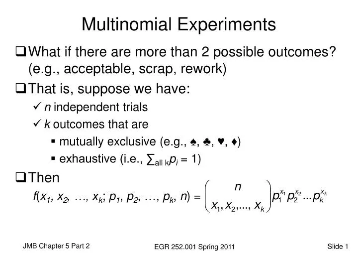
Multinomial Experiments. What if there are more than 2 possible outcomes? (e.g., acceptable, scrap, rework) That is, suppose we have: n independent trials k outcomes that are mutually exclusive (e.g., ♠, ♣, ♥, ♦) exhaustive (i.e., ∑ all k p i = 1) Then

E N D
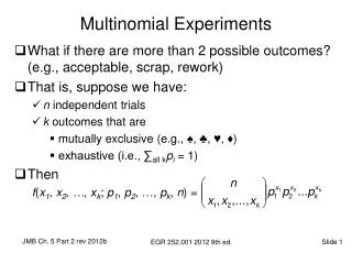
Multinomial Experiments • What if there are more than 2 possible outcomes? (e.g., acceptable, scrap, rework) • That is, suppose we have: • n independent trials • k outcomes that are • mutually exclusive (e.g., ♠, ♣, ♥, ♦) • exhaustive (i.e., ∑all kpi = 1) • Then f(x1, x2, …, xk; p1, p2, …, pk, n) = EGR 252.001 Spring 2011
Problem 22, pg. 152 • Convert ratio 8:4:4 to probabilities • f( __, __, __; ___, ___, ___, __) =_______ • f( 5,2,1; 0.5, 0.25, 0.25, 8) • = (8 choose 5,2,1)(0.5)5(0.25)2(0.25)1 • = 8!/(5!2!1!)* )(0.5)5(0.25)2(0.25)1 • = 21/256 or 0.082031 EGR 252.001 Spring 2011
Binomial vs.Hypergeometric Distribution • Replacement and Independence • Binomial (assumes sampling “with replacement”) and hypergeometric (sampling “without replacement”) • Binomial assumes independence, while hypergeometric does not. • Hypergeometric: The probability associated with getting x successes in the sample (given k successes in the lot.) EGR 252.001 Spring 2011
Hypergeometric Example • Example from Complete Business Statistics, 4th ed (McGraw-Hill) • Automobiles arrive in a dealership in lots of 10. Five out of each 10 are inspected. For one lot, it is known that 2 out of 10 do not meet prescribed safety standards. What is probability that at least 1 out of the 5 tested from that lot will be found not meeting safety standards? • This example follows a hypergeometric distribution: • A random sample of size n is selected without replacement from N items. • k of the N items may be classified as “successes” and N-k are “failures.” • The probability associated with getting x successes in the sample (given k successes in the lot.) EGR 252.001 Spring 2011
Solution: Hypergeometric Example • In our example, k = number of “successes” = 2 n = number in sample = 5 N = the lot size = 10 x = number found = 1 or 2 P(X > 1) = 0.556 + 0.222 = 0.778 EGR 252.001 Spring 2011
Expectations: Hypergeometric Distribution • The mean and variance of the hypergeometric distribution are given by • What are the expected number of cars that fail inspection in our example? What is the standard deviation? μ = nk/N = 5*2/10 = 1 σ2 =(5/9)(5*2/10)(1-2/10) = 0.444 σ =0.667 EGR 252.001 Spring 2011
Your turn … A worn machine tool produced defective parts for a period of time before the problem was discovered. Normal sampling of each lot of 20 parts involves testing 6 parts and rejecting the lot if 2 or more are defective. If a lot from the worn tool contains 3 defective parts: • What is the expected number of defective parts in a sample of six from the lot? N = 20 n = 6 k = 3μ = nk/N = 6*3/20 =18/20=0.9 • What is the expected variance? σ2 = (14/19)(6*3/20)(1-3/20) = 0.5637 • What is the probability that the lot will be rejected? P(X>2) = 1 – [P(0)+P(1)] EGR 252.001 Spring 2011
Binomial Approximation • Note, if N >> n, then we can approximate the hypergeometric with the binomial distribution. • Example: Automobiles arrive in a dealership in lots of 100. 5 out of each 100 are inspected. 2 /10 (p=0.2) are indeed below safety standards. What is probability that at least 1 out of 5 will be found not meeting safety standards? • Recall: P(X≥ 1) = 1 – P(X< 1) = 1 – P(X = 0) (Compare to example 5.14, pg. 129) EGR 252.001 Spring 2011
Negative Binomial Distribution b* • A binomial experiment in which trials are repeated until a fixed number of successes occur. • Example: Historical data indicates that 30% of all bits transmitted through a digital transmission channel are received in error. An engineer is running an experiment to try to classify these errors, and will start by gathering data on the first 10 errors encountered. What is the probability that the 10th error will occur on the 25th trial? EGR 252.001 Spring 2011
Negative Binomial Example • This example follows a negative binomial distribution: • Repeated independent trials. • Probability of success = p and probability of failure = q = 1-p. • Random variable, X, is the number of the trial on which the kth success occurs. • The probability associated with the kth success occurring on trial x is given by, Where, k = “success number” = 10 x = trial number on which k occurs = 25 p = probability of success (error) = 0.3 q = 1 – p= 0.7 EGR 252.001 Spring 2011
Negative Binomial Distribution • In our example, k = “success number” = 10 x = trial number on which k occurs = 25 p = probability of success (error) = 0.3 q = 1 – p= 0.7 EGR 252.001 Spring 2011
Geometric Distribution • Example: In our example, what is the probability that the 1st bit received in error will occur on the 5th trial? • This is an example of the geometric distribution, which is a special case of the negative binomial in which k = 1. • The probability associated with the 1st success occurring on trial x is given by = (0.3)(0.7)4 = 0.072 EGR 252.001 Spring 2011
Your turn … A worn machine tool produces 1% defective parts. If we assume that parts produced are independent: • What is the probability that the 2nd defective part will be the 6th one produced? • What is the probability that the 1st defective part will be seen before 3 are produced? • How many parts can we expect to produce before we see the 1st defective part? (Hint: see Theorem 5.4, pg. 161) EGR 252.001 Spring 2011
Poisson Process • The number of occurrences in a given interval or region with the following properties: • “memoryless” ie number in one interval is independent of the number in a different interval • P(occurrence) during a very short interval or small region is proportional to the size of the interval and doesn’t depend on number occurring outside the region or interval. • P(X>1) in a very short interval is negligible EGR 252.001 Spring 2011
Poisson Process Situations • Number of bits transmitted per minute. • Number of calls to customer service in an hour. • Number of bacteria present in a given sample. • Number of hurricanes per year in a given region. EGR 252.001 Spring 2011
Service Call Example - Poisson Process • Example An average of 2.7 service calls per minute are received at a particular maintenance center. The calls correspond to a Poisson process. To determine personnel and equipment needs to maintain a desired level of service, the plant manager needs to be able to determine the probabilities associated with numbers of service calls. EGR 252.001 Spring 2011
Poisson Distribution Probabilities • The probability associated with the number of occurrences in a given period of time is given by, Where, λ= average number of outcomes per unit time or region t = time interval or region EGR 252.001 Spring 2011
Our Example: λ= 2.7 and t = 1 minute • What is the probability that fewer than 2 calls will be received in any given minute? • The probability that fewer than 2 calls will be received in any given minute is P(X < 2) =P(X = 0) + P(X = 1) • The mean and variance are both λt, so μ = λt =________________ • Note: Table A.2, pp. 748-749, gives Σtp(x;μ) EGR 252.001 Spring 2011
Service Call Example - Part 2 • If more than 6 calls are received in a 3-minute period, an extra service technician will be needed to maintain the desired level of service. What is the probability of that happening? • μ = λt = (2.7) (3)= 8.4 • 8.4 is not in the table; use basic equation • Supposeλt = 8; see table with μ = 8 and r = 6 P(X > 6) = 1 – P(X <6) = 1 - 0.3134 = 0.6866 EGR 252.001 Spring 2011
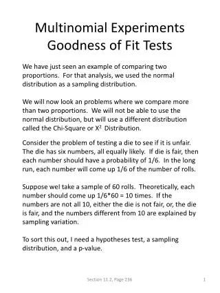
Poisson Distribution EGR 252.001 Spring 2011
Poisson Distribution The effect of λ on the Poisson distribution EGR 252.001 Spring 2011