Download
1 / 18
180 likes | 268 Vues
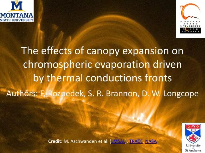
The effects of canopy expansion on chromospheric evaporation driven by thermal conductions fronts. Authors: F. Rozpedek , S . R. Brannon, D. W. Longcope. Credit: M. Aschwanden et al. ( LMSAL ), TRACE , NASA. Abstract.

E N D
The effects of canopy expansion on chromospheric evaporation driven by thermal conductions fronts Authors: F. Rozpedek, S. R. Brannon, D. W. Longcope Credit: M. Aschwanden et al. (LMSAL), TRACE, NASA
Abstract The solar corona is well known for its highly structured appearance. This structuring is partly due to its magnetic field, and partly due to the complex distribution of mass within the field. Coronal mass density is set by coronal heating which might be constant (the steady-heating picture) or might be sporadic (the so-called nanoflare picture). In the latter scenario, a mass flux occurs through a process referred to as chromospheric evaporation. Reconnection and subsequent loop contraction generate shocks in the corona which result in thermal conduction fronts. These fronts impulsively deposit heat into the cooler chromosphere and drive supersonic upward flows which is the evaporation. This process has been extensively studied in the past, but generally using models with uniform magnetic field connecting the corona and chromosphere. Transonic flows are known, in general, to be highly sensitive to variation in the cross-section through which they are driven. It is therefore expected that the complex structure of the magnetic canopy could have a dramatic effect on the supply of mass into the corona. We explore this possibility using a simplified 1-D hydrodynamic model of evaporation occurring through a varying magnetic field canopy.
Observed Data Observed flow velocities () at various temperatures (squares) for a C4.2-class flare (Li & Ding 2011). Dashed line is a linear fit of vs. Note the high temperature (6.3 MK) conversion between up- and down-flows which is incompatible with particle beams but consistent with thermal conduction fronts (TCFs).
Shocktube Model • The above picture illustrates the uniform shocktube, • The shock is generated by the piston moving down the tube with the speed Mpiston= 3.0 (the piston moves outside the simulation region), • Our simulation establishes the time evolution of pressure, fluid velocity, density and temperature in the Chromosphere, Transition Region (TR) and the Corona, • The loop atmosphere includes uniform coronal and chromospheric temperatures connected by a TR of uniform pressure and with temperature gradient of the form: where is the ratio of coronal to chromospheric temperatures, is the length scale of the TR and is its position, • At equilibrium, the temperature gradient between the Corona and the Chromosphere is maintained by the term , where is the distance along the tube. This term corresponds to “Coronal Heating” and “Chromospheric Radiation”, • All quantities are scaled to the coronal values, the model does not include gravity and explicit radiation.
Time Evolution for the uniform tube On the left: time evolution of pre-ssure, fluid velocity, density and tempera-ture in the uniform shocktube. Pressure peak generates up- and down-flows. E C VRP E C Evaporation C Condensation E TCF Thermal Con- duction Front TCF Velocity re- versal point VRP
The “Canopy” Model On the left: Top view, imaginary sources of magnetic field in the photosphere, their distribution results in the “nozzle” shape of the fluxtube area profile. The red dashed line marks the cross-section for the picture below. Letters “A”, “B” and “C” mark the position of the corresponding vertical lines labeled on the picture below. A C B On the right: Side view, magnetic field lines coming out of the monopole P001. The shape of this cross-section of the fluxtube is determined by the influence of the neighboring monopoles P011 (fieldline C) and P004 (fieldline A).
Varying Area Profile Nozzle below the TR Nozzle above the TR Nozzle at the centre of the TR The area profile is of the same functional form as the temperature profile.
Effect of the nozzle on the TCF without atmosphere Time evolution of the Temperature in the atmosphere-free shocktube for: a) a uniform tube, b) a tube with the nozzle at 0.25, c) a tube with the nozzle at 0.35. Note that TCF speeds up and the slope steepens at the front as it moves through the nozzle.
Temperature Evolution Energy Equation: For atmosphere-free case: In 1-D: Hence the Energy Equation becomes: And can be rewritten as: Normal diffusion is enhanced by effective thermal velocity The result of that is the steepening of the temperature gradient and acceleration of the TCF.
Velocity Reversal Point Velocity Reversal Point (VRP) occurs on the border of where the condensation region turns into the evaporation region Below: An example graph of fluid velocity vs with VRP and the slope at VRP clearly marked. VRP Above: Fluid Velocity vs Temperature in a uniform tube plotted for different time frames. Note that VRP tends to move down in T during early development of the evaporation.
Velocity Reversal Point On the left: Temperature at the Velocity Reversal Point as a function of time for the area profile with the nozzle placed at 0.25. Note that there is a local minimum of between Frames 130 and 150. We will call that time t0. On the right: Slope of velocity versus graph at the Velocity Reversal Point plotted as a function of time for the area profile with the nozzle placed at 0.25.
Velocity Reversal Point One can also find the time t0 for which the temperature at the Velocity Reversal Point is locally at its minimum (as marked on the previous slide). We choose the minimum lying in the time interval for which the temperature doesn’t change rapidly with time, as that interval corresponds to what happens after the evaporation has already started. Then this minimum temperature and the slope on the velocity versus graph at the Velocity Reversal Point at that time t0 are plotted as a function of the nozzle location. This temperature dependence is shown on the plot above and the corresponding derivative on the graph on the left.
Velocity Reversal Point Above: time t0 as a function of the position of the nozzle.
Filling of the Loop during Evaporation To investigate the extend to which the chromospheric evaporation can fill the loop, various quantities have been calculated. The first one is the total mass moving up the loop: On the left: The total mass flowing up the loop averaged over the time of the simulation plotted as a function of the position of the nozzle.
Filling of the Loop during Evaporation Since the total mass flowing up does not take into account how quickly this mass is moving, another quantity which is useful in examining the filling of the loop is the total momentum up On the left: The total upward momentum averaged over the time of the simulation plotted as a function of the position of the nozzle.
Filling of the Loop during Evaporation Another measure of filling of the loop could be based on calculating the difference of densities between the density at a given time and the initial density for the points where this difference is positive. As it is only evaporation that is responsible for filling of the loop, our calculation excludes the condensation region. On the left: to measure how quickly the loop is filled, the Relative Loop Filling (t1)/ t1, [where t1 is the duration of the simulation] has been plotted as a function of the position of the nozzle.
Comments Discussion Future Work Investigation of the functional dependence on the position of the nozzle of: a) temperature at VRP, b) time at VRP, c) slope on the velocity versus graph at VRP. Simulations and investigation of variation of other parameters of the nozzle-shape area profile, that is the length of the nozzle and the fractional change in area at the nozzle. Development of a model to accommodate observational data in a systematic fashion. • The simulations with nozzle placed at various positions and without atmosphere show that TCF accelerates after encountering the nozzle (it encounters a narrowing in the area). Moreover, the forward portion of the TCF is steeper on the temperature vs position plot. • However, the temperature and time at VRP vs position of the nozzle are not monotonic as we would expect from the above observations (temperature is not everywhere increasing and time is not everywhere decreasing). Hence this must be due to some additional effects of the atmosphere on the evaporation.
References: • Fisher, G. H., Canfield, R. C. and McClymont, A. N. "Flare Loop Radiative Hydrodynamics. V - Response to Thick-target Heating." The Astrophysical Journal 289 (1985): 414-24. Print. • Li, Y., and Ding, M. D. "Different Patterns of Chromospheric Evaporation in a Flaring Region Observed with Hinode/EIS." The Astrophysical Journal 727 (2011): 98. Print. • MacNeice, P. "A Numerical Hydrodynamic Model of a Heated Coronal Loop." Solar Physics 103.1 (1986): 47-66. Print. • Milligan, R. O. "Spatially Resolved Nonthermal Line Broadening During The Impulsive Phase Of A Solar Flare." The Astrophysical Journal 740.2 (2011): 70. Print. • Nagai, F. "A Model of Hot Loops Associated with Solar Flares." Solar Physics 68.2 (1980): 351-79. Print. • Acknowledgements: • The authors would like to thank MSU Solar Physics REU Program, as well as Prof. Eric Priest for his valuable comments.