Download
1 / 30
300 likes | 602 Vues
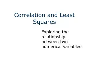
Correlation and Least Squares. Exploring the relationship between two numerical variables. Preview of Remainder of Course. So far we have: Discussed sampling methods and study designs Talked about inference for proportions Talked about inferences for means

E N D
Correlation and Least Squares Exploring the relationship between two numerical variables.
Preview of Remainder of Course • So far we have: • Discussed sampling methods and study designs • Talked about inference for proportions • Talked about inferences for means • Now we will go into the bi-variate numerical and multi-variate numerical worlds and attempt to mathematically describe relationships between different variables
Preview of Remainder of Course • For example, is there a relationship between people’s heights and hand spans? It makes sense that taller people tend to have greater hand spans than shorter people. But to what extent? How reliable is this generalization? Is there an equation to describe this relationship? If there is such an equation, how reliable is it? How well does the equation match up to the real world? These are the types of questions we will attempt to address.
Introduction to Bivariate Data • We will start with the simpler case: bi-variate data • We measure (x,y) on each individual • Examples: (height, hand span), (study hours, GPA), (auto mileage, auto price) • Names for x: predictor, independent variable, factor • Names for y: response, dependent variable • Goal: find an equation y = f(x) + e, where e is an error term, to describe the relationship
Scatter Plots • We measure (x,y) on each individual • We represent each individual as a point on an x-y plot • The resulting graph is a scatter plot. • Example: Measure x = height (in) and measure y = hand span (cm) • The plot is titled Y vs. X.
Some Important Questions • Examine the scatter plot to look for important information. • Would a straight line summarize the results well? • Would a parabola summarize the results well? • Does the variability in Y depend on the value of X?
Hand Span vs. Height The relationship between the hand span and height would be summarized well by a straight line. The variation in Y appears constant across values of X. Yield vs. Date A parabola would summarize the relationship between yield and date. The variation in Y appears constant across values of X. The Two Scatter Plots
Correlation • The strength (and nature) of linear trends is described with a numerical measure called correlation. • The sign of the correlation indicates the nature of the relationship: positive or negative (the sign of the slope of the line). • The magnitude of the correlation indicates the strength of the relationship: • correlation = 0 means no (linear) relationship • correlation = 1 means the points fall EXACTLY on a straight line
Sample correlation = r Pop corr. = r (“rho”) -1 r 1 & -1 r 1 High magnitude of correlation indicates a strong mathematical relationship – NOT necessarily a cause and effect relationship. Measures only the strength of LINEAR relationships - not other types of relationships Does not depend on units that are used r itself is unitless Notation and Properties
Hand Span vs. Height • The sample correlation is r = 0 .8767. • This indicates a strong positive linear relationship. • As height increases, hand span increases in a linear fashion.
Crab Meat Weight vs. Total Weight • r = 0.8679 • This indicates a strong positive linear relationship between total weight and meat weight. • As the total weight increases, so does the meat weight.
Bacterial Growth vs. C02 Level • r = -0.9117 • A strong negative relationship. • As C02 increases, the bacterial growth decreases. • However, the relationship is somewhat curved, not LINEAR.
A Semicircle • r = 0, even though an obvious relationship is present. • Correlation measures LINEAR relationships.
Part of a Parabola • r = 0.9653 • Even though the relationship is not linear, a straight line with positive slope fits fairly well. • However, a line should NOT be used to summarize this data.
Correlation Properties • Correlation is always between -1 and 1. • A positive correlation indicates that if a relationship is linear, it is positive (as x increases, so does y). • A negative correlation indicates that if a relationship is linear, it is negative (as x increases, y decreases).
Correlation Properties • A strong correlation does not necessarily mean that x and y are involved in a cause and effect relationship. • A strong correlation does not mean that the best description of the relationship between x and y is a linear one. It simply means a linear relationship describes the relationship well. • A weak correlation does not mean a relationship does not exist. It simply means that if a relationship exists, it is not a strong linear relationship. In fact, there may be a very strong nonlinear relationship.
Dealing with bivariate or multivariate data Started with bivariate data Describe with a scatter plot (plot of (x,y) points) Correlation developed for LINEAR trends Suppose we do have a linear trend, what next? Find equation for line Characterize its reliability Relate sample line to population line Use line to make predictions Review So Far & What’s Ahead
The Method of Least Squares • Suppose we believe that the relationship between x and y is linear. • We specify that the population relationship is of the form y = b0 +b1 x + e. • The method of least squares is used to find the sample based estimate y = b0 + b1 x + e. • The basic idea is to find values of b0 and b1 to minimize the sum of squared errors (in y).
Uses calculus to find values for the sample slope and intercept to minimize the estimated sum of squared errors If the true pop errors are normal, the estimates of the slope and intercept are normal. This property lets us use t-based procedures to perform hypothesis tests and form CI’s for the slope and intercept. Results hold for populations with non-normal errors if we have large sample. However, least squares is very sensitive to outliers. Method of Least Squares
Method of Least Squares • Without outliers, the method of least squares yields a line that is a good description of the relationship between hand span and height. • However, adding two outliers (wide span, short) and (narrow span, tall) makes the line almost horizontal. • These two points completely reconfigure the line.
Regression • Regression is using the method of least squares is to estimate a mathematical relationship between two (or more) variables. • Regression is used to make predictions about a population (or even an individual) based on a sample. • When the relationship is a straight line, it is called simple linear regression.
Regression Example • For the hand span and height data, the least squares estimated line is span (cm) = -14.01 + 0.51 height (in). • Give me a height, and I’ll give you a good estimate of the mean span of the population of individuals of that height (by plugging in). • If height = 70 inches, span = -14.01 + 0.51 70 = 21.69. • It is important to use the correct units. • This is an estimate. To use regression for prediction, we’ll need an interval estimate.
Regression gives a lot of useful information besides just the equation for the line Adjusted R2 = proportion of variation in y explainable by x Span-Height adjR2 = 0.74 74% of variation in hand-span explained by height Root Mean Squared Error (RMSE) is the standard deviation of the residuals (sample estimates of error) RMSE = 1.16 So the standard deviation of points (in y) around the line is 1.16. A good fit is indicated by high adjusted R2 and low RMSE! Regression Example
Goal: find and/or estimate a mathematical relationship between y and x Scatterplot (x,y) Correlation measures strength and nature of LINEAR relationship Method of least squares minimizes sum of squared errors Using least squares to find form of equation is called regression Regression also gives adjusted R2 and RMSE Review of Today
If these conditions hold Independence Normal errors Errors have mean zero Errors have equal SD Then we can Find CI’s for the slope and intercept Find a CI for the mean of y at a given x Find a prediction interval (PI) for an individual y at a given x Preview of Next Time