Download
1 / 29
290 likes | 466 Vues
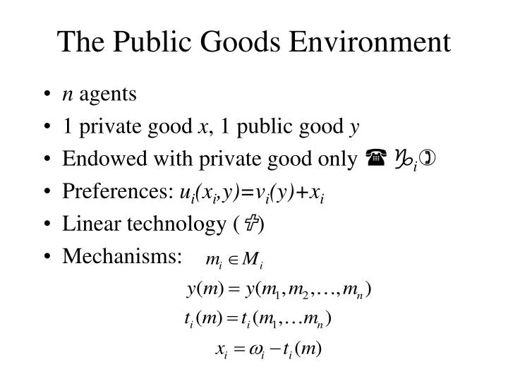
The Public Goods Environment. n agents 1 private good x , 1 public good y Endowed with private good only ( g i ) Preferences: u i (x i ,y)=v i (y)+x i Linear technology ( ) Mechanisms:. Five Mechanisms . “Efficient” => g ( e ) PO ( e ) Inefficient Mechanisms

E N D
The Public Goods Environment • n agents • 1 private good x, 1 public good y • Endowed with private good only (gi) • Preferences: ui(xi,y)=vi(y)+xi • Linear technology () • Mechanisms:
Five Mechanisms • “Efficient” => g(e) PO(e) • Inefficient Mechanisms • Voluntary Contribution Mech. (VCM) • Proportional Tax Mech. • (Outcome-) Efficient Mechanisms • Dominant Strategy Equilibrium • Vickrey, Clarke, Groves (VCG) (1961, 71, 73) • Nash Equilibrium • Groves-Ledyard (1977) • Walker (1981)
The Experimental Environment • n = 5 • Four sessions of each mech. • 50 periods (repetitions) • Quadratic, quasilinear utility • Preferences are private info • Payoff ≈ $25 for 1.5 hours • Computerized, anonymous • Caltech undergrads • Inexperienced subjects • History window • “What-If Scenario Analyzer”
What-If Scenario Analyzer • An interactive payoff table • Subjects understand how strategies → outcomes • Used extensively by all subjects
Environment Parameters • Loosely based on Chen & Plott ’96 • = 100 • Pareto optimum: yo =(bi - )/(2ai)=4.8095
Voluntary Contribution Mechanism Mi = [0,6] y(m) = imi ti(m)= mi • Previous experiments: • All players have dominant strategy: m* = 0 • Contributions decline in time • Current experiment: • Players 1, 3, 4, 5 have dom. strat.: m* = 0 • Player 2’s best response: m2* = 1 - i2mi • Nash equilibrium: (0,1,0,0,0)
VCM Results Nash Equilibrium: (0,1,0,0,0) Dominant Strategies Player 2
Proportional Tax Mechanism Mi = [0,6] y(m) = imi ti(m)=(/n)y(m) • No previous experiments (?) • Foundation of many efficient mechanisms • Current experiment: • No dominant strategies • Best response: mi* = yi*ki mk • (y1*,…,y5*) = (7, 6, 5, 4, 3) • Nash equilibrium: (6,0,0,0,0)
Prop. Tax Results Player 1 Player 2
Groves-Ledyard Mechanism • Theory: • Pareto optimal equilibrium, not Lindahl • Supermodular if /n > 2aifor every i • Previous experiments: • Chen & Plott ’96 – higher => converges better • Current experiment: • =100 => Supermodular • Nash equilibrium: (1.00, 1.15, 0.97, 0.86, 0.82)
Walker’s Mechanism • Theory: • Implements Lindahl Allocations • Individually rational (nice!) • Previous experiments: • Chen & Tang ’98 – unstable • Current experiment: • Nash equilibrium: (12.28, -1.44, -6.78, -2.2, 2.94)
Walker Mechanism Results NE: (12.28, -1.44, -6.78, -2.2, 2.94)
VCG Mechanism: Theory • Truth-telling is a dominant strategy • Pareto optimal public good level • Not budget balanced • Not always individually rational
VCG Mechanism: Best Responses • Truth-telling ( ) is a weak dominant strategy • There is always a continuum of best responses:
VCG Mechanism: Previous Experiments • Attiyeh, Franciosi & Isaac ’00 • Binary public good: weak dominant strategy • Value revelation around 15%, no convergence • Cason, Saijo, Sjostrom & Yamato ’03 • Binary public good: • 50% revelation • Many pairings play dominated Nash equilibria • Continuous public good with single-peaked preferences (strict dominant strategy): • 81% revelation
VCG Experiment Results • Demand revelation: 50 – 60% • NEVER observe the dominant strategy equilibrium • 10/20 subjects fully reveal in 9/10 final periods • “Fully reveal” = both parameters • 6/20 subjects fully reveal < 10% of time • Outcomes very close to Pareto optimal • Announcements may be near non-revealing best responses
Summary of Experimental Results • VCM: convergence to dominant strategies • Prop Tax: non-equil., but near best response • Groves-Ledyard: convergence to stable equil. • Walker: no convergence to unstable equilibrium • VCG: low revelation, but high efficiency Goal: A simple model of behavior to explain/predict which mechanisms converge to equilibrium Observation: Results are qualitatively similar to best response predictions
A Class of Best Response Models • A general best response framework: • Predictions map histories into strategies • Agents best respond to their predictions • A k-period best response model: • Pure strategies only • Convex strategy space • Rational behavior, inconsistent predictions
Testable Predictions of the k-Period Model • No strictly dominated strategies after period k • Same strategy k+1 times => Nash equilibrium • U.H.C. + Convergence to m* => m* is a N.E. 3.1. Asymptotically stable points are N.E. • Stability: 4.1. Global stability in supermodular games 4.2. Global stability in games with dominant diagonal Note: Stability properties are not monotonic in k
Choosing the best k • Which k minimizest |mtobs mtpred| ? • k=5 is the best fit
Statistical Tests: 5-B.R. vs. Equilibrium • Null Hypothesis: • Non-stationarity => period-by-period tests • Non-normality of errors => non-parametric tests • Permutation test with 2,000 sample permutations • Problem: If then the test has little power • Solution: • Estimate test power as a function of • Perform the test on the data only where power is sufficiently large.
5-period B.R. vs. Nash Equilibrium • Voluntary Contribution (strict dom. strats): • Groves-Ledyard (stable Nash equil): • Walker (unstable Nash equil): 73/81 tests reject H0 • No apparent pattern of results across time • Proportional Tax: 16/19 tests reject H0 • 5-period model beats any static prediction
Best Response in the VCG Mechanism • Convert data to polar coordinates:
Best Response in the cVCG Mechanism Origin = Truth-telling dominant strategy 0-degree Line = Best response to 5-period average
Efficiency Efficiency Confidence Intervals - All 50 Periods 1 Efficiency No Pub Good 0.5 Walker VC PT GL VCG Mechanism
The Testable Predictions • Weakly dominated ε-Nash equilibria are observed (67%) • The dominant strategy equilibrium is not (0%) • Convergence to strict dominant strategies 2,3. 6 repetitions of a strategy implies ε-equilibrium (75%) • Convergence with supermodularity & dom. diagonal (G-L)
Conclusions • Importance of dynamics & stability • Dynamic models outperform static models • Strict vs. weak dominant strategies • Applications for “real world” implementation • Directions for theoretical work: • Developing stable mechanisms • Open experimental questions: • Efficiency/equilibrium tension in VCG • Effect of the “What-If Scenario Analyzer” • Better learning models