Download
1 / 46
460 likes | 609 Vues
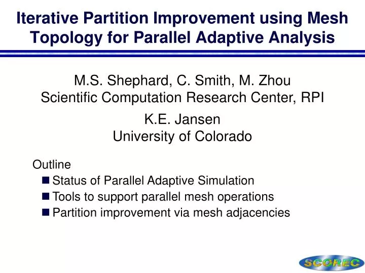
Iterative Partition Improvement using Mesh Topology for Parallel Adaptive Analysis. M.S. Shephard , C. Smith, M. Zhou Scientific Computation Research Center, RPI K .E. Jansen University of Colorado. Outline Status of Parallel Adaptive Simulation

E N D
Iterative Partition Improvement using Mesh Topology for Parallel Adaptive Analysis M.S. Shephard, C. Smith, M. ZhouScientific Computation Research Center, RPI K.E. Jansen University of Colorado • Outline • Status of Parallel Adaptive Simulation • Tools to support parallel mesh operations • Partition improvement via mesh adjacencies
Parallel Adaptive Analysis • Components • Solver • Form the system of equations • Solve the system of equations • Parallel mesh representation/manipulation • Partitioned mesh management • Mesh adaptation procedure • Driven by error estimates and/or correction indicators • Mesh improvement procedures • Dynamic load balancing • Need to regain load balance • All components must operate in parallel • Prefer to exercise parallel control of all operations with same overall parallel structure – improves scalability initial mesh adapted mesh
Parallel Adaptive Analysis Tools Used • An implicit stabilized finite element code (PHASTA) • Supports simulations on general unstructured meshes including boundary layers and anisotropic meshes • Stabilized methods can provide high order convergence while maintaining good numerical properties • Equations solved using iterative methods • Parallel mesh representation/manipulation • ITAPS iMeshP/FMDB • Utilities for partition management and predictive load balancing • Mesh adaptation based on mesh modification • Avoid the accuracy and data problems associated with full remeshing • With sufficient number of modification operators and control algorithms mesh modification can support general changes to the mesh • “Graph-based” dynamic load balancing • Classic partition graph for initial distribution • Graph defined by mesh topology for partition improvement
… NS Flow Solver • Implicit non-linear FEM solver with two phases of computation: • Equation formation (Eqn. form.) – depends on elements • Equation solution – depends on degrees-of-freedom (dofs): Weak form – Defined as sum of element integrals Quadrature – Simply adds loop inside element loop Assembly – As elements processes element matrices and vectors processes Iterative solver
Eqn. sol. Eqn. form. PartC PartA PartB PartC PartA PartB during Eqn. form. during Eqn. sol. Parallelization • Parallel strategy: • Both compute stages operate off the same mesh partition – critical to scalability • Partition defines inter-part relations (part-to-part comm.) Locally, incomplete values (in b, A, q, etc.)for shared dofs. Apply communications to complete values/entries (in b, q only)
dofs are shared between parts control relationship between images (solid dots indicate owner images) PartA PartB values accumulated on owners values updated on to non-owners PartC Current Approach – Parallelization • Communications to complete values/entries and norms (same overall calculations as methods based on global matrix): complete b complete q (for on-part q=Ap) on-part norm for q and all-reduce (use complete q)
Parallel Implicit Flow Solver – IncompressibleAbdominal Aorta Aneurysm (AAA) 105 Million Elements 32K parts show modest degradation due to 15% node imbalance (with only about 600 mesh-nodes/part) Rgn./elem. ratioi = rgnsi/avg_rgns Node ratioi = nodesi/avg_nodes
comm-to-comp ratio increases Strong Scaling – 1B Mesh up to 160k Cores • AAA 1B elements: further scaling analysis (ttot=tcomm+tcomp)
Strong Scaling – 1B Mesh up to 288k Cores • AAA 1B elements: three supercomputers up to full-system scale 18.67 on XT5 and 14.39 on BGP secs for 20 time steps
Strong Scaling – 5B Mesh up to 288k Cores • AAA 5B elements: full-system scale on Jugene (IBM BG/P) without PIMA strong scaling factor is 0.88 (time is 70.5 secs), for production runs savings can be in 43 cpu-years
initial mesh (20,067 tets) adapted mesh (approx. 2M tets) Edge collapse Edge split face split Double split collapse to remove the red sliver Mesh Adaptation by Local Mesh Modification • Controlled application of mesh modification operations including dealing with curved geometries, anisotropic meshes • Base operators • swap • collapse • Split • move • Compound operators chain single step operators • Double split collapse operator • Swap(s) followed by collapse operator • Split, then move the created vertex • Etc.
Matching Boundary Layer and Interior Mesh • A modification operation on any layer is propagated through the stack and interface elements to preserve attributes of layered elements.
Parallel Mesh Adaptation • Parallelization of refinement: perform on each part and synchronize at inter-part boundaries. • Parallelization of coarsening and swapping: migrate cavity (on-the-fly) and perform operation locally on one part. • Support for parallel mesh modification requires update of evolving communication-links between parts and dynamic mesh partitioning.
t=0.0 t=2e-4 t=5e-4 Adaptive Loop Construction • Tightly coupled • Adv: Computationally efficient if done well • Disadv: More complex code development • Example: Explicit solution of cannon blasts • Loosely coupled • Adv: Ability to use existing analysis codes • Disadv: Overhead of multiple structures and data conversion • Example: Implicit high-orderFE code developed by DOEfor EM simulations of linear accelerators
The initial mesh has 7.1 million regions The local size mesh size is between 0.03cm and 0.1cm The initial mesh is isotropic Initial mesh BL with 0.004cm as the height of each Patient Specific Vascular Surgical Planning
4 mesh adaptation iterations The adapted mesh:42.8 million regions 7.1M->10.8M->21.2M->33.0M->42.8M Boundary layer based mesh adaptation Mesh is anisotropic The minimum local size: 0.004cm, maximum local size: 0.8cm, and the height of the boundary layer: 0.004cm. Note: the inflow diameter is 3cm, and the total model length is more than 150cm. Mesh adaptation driven by 2nd derivatives of appropriate solution field (velocity and pressure in current case) Patient Specific Vascular Surgical Planning Brain-left Spleen SMA Anisotropic adapted mesh
Parallel Boundary Layer Adaptation Initial mesh of 450k elements Final mesh of 4.5m elements
Parallel Boundary Layer Adaptation Initial mesh of 450k elements Final mesh of 4.5m elements
Parallel Boundary Layer Adaptation Initial mesh of 450k elements Final mesh of 4.5m elements
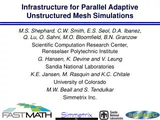
Tools to Support Parallel Mesh Operations • Unstructured mesh tools used to support parallel adaptive analysis on massively parallel computers • Distributed mesh representation • Mesh migration • Dynamic load balancing • Multiple parts per process • Predictive load balancing • Partition improvement
partition boundary P 0 P 2 1 M j 0 M i P 1 Distributed Mesh Data Structure • Distributed Mesh • Mesh divided into parts for distribution onto nodes/cores • Part Pi consists of mesh entities assigned to the ith part. • Partition Object • Basic unit assigned to a part • A mesh entity to be partitioned • An entity set (where the set of entities are required to be kepton the same part). • Residence Part • Operator P [Mid] returns a set of part id’s where Mid exists. (e.g. P [M10] = {P0, P1, P2} )
A Partition Model • Interoperable partition model implementation - iMeshP • Defined by the DOE SciDAC center on Interoperable tools for Advanced Petascale Simulations • Supports unstructured meshes on distributed memory parallel computers • Focuses on supporting parallel interactions of serial (iMesh) on part meshes • Multiple implementations underway • Implementation that support parallel mesh adaptation used here.
Mesh Migration • Movement of mesh entities between parts • Dictated by operation - in swap and collapse it’s the mesh entities on other parts needed to complete the mesh modification cavity • Information determined based on mesh adjacencies • Complexity of mesh migration a function of mesh representation • Complete representation can provide any adjacency without mesh traversal - a requirement for satisfactory efficiency • Both full and reduced representations can be complete • Full representation - all mesh entities explicitly represented • Reduced representation - requires all mesh vertices and mesh entities of the same order as the model (or partition) entity they are classified on
Dynamic Partitioning of Unstructured Meshes • Load balance is lost during mesh modification • Need to rebalance in parallel on already distributed mesh • Want equal “work load” with minimum inter-processor communications • Graph based methods are flexible and provide best results • Zoltan Dynamic Services (http://www.cs.sandia.gov/Zoltan/) • Supports multiple dynamic partitioners • General control of the definition of part objects and weights supported • Under active development
Multiple Parts per Process • Support more that one part per process • Key to changing number of parts • Also used to deal with problem with current graph-based partitioners that tend to fail on really large numbers of processors • 1 Billion region mesh starts as well balanced mesh on 2048 parts • Each part splits to 64 parts - get 128K parts via ‘local’ partitioning • Region imbalance: 1.0549 • Time usage < 3mins on Kraken • This is the partition used for scaling test on Intrepid
Multiple Parts per Process • Supports global and local graphs to create mesh partitions at extreme scale (>=100K parts): Global partition Global graph Mesh and its initial partition (partition from 3 parts to 6 parts) Local graph Local partition
Predictive Load Balancing • Mesh modification before load balancing can lead to memory problems • Employ predictive load balancing to avoid the problem • Assign weights based on what will be refined/coarsened • Apply dynamic load balancing using those weights • Perform mesh modifications • May want to do some local migration
Algorithm Mesh metric field at any point P is decomposed to three unit direction (e1,e2,e3) and desired length (h1,h2,h3) in each corresponding direction. The volume of desired element (tetrahedron) : h1h2h3/6 Estimate number of elements to be generated: “num” is scaled to a good range before it is specified as a weight to graph nodes Predictive Load Balancing ? # regions ?
Predictive Load Balancing Initial: 8.7M; Adapted: 80.5M PredL run on 128 cores Initial: 8.7M; Adapted: 187M Test run out of memory without PredLB on 200 cores
Partitioning Improvement via Mesh Adjacencies • Observations on graph-based dynamic balancing • Parallel construction and balancing of graph with small cuts takes reasonable time • In the case of unstructured meshes, the graph defined in terms of • Graph nodes as mesh entity type to be balanced (e.g., regions, faces, edges or vertices) • Graph edges based on mesh adjacencies taken into account (e.g., graph edge between regions sharing a vertex, between regions sharing a face, etc.) • Accounting for multiple criteria and or multiple interactions is not obvious • Hypergraphs allows edges to connect more that two vertices may be of use – has been used to help account for migration communication costs
Partition Improvement via Mesh Adjacencies • Mesh adjacencies for a complete representation can be viewed as a complete graph • All entities can be “graph-nodes” at will • Any desired graph edge obtained in O(1) time • Possible advantages • Avoid graph construction (assuming you have needed adjacencies) • Account for multiple entity types – important for the solve process - typically the most computationally expensive step • Disadvantage • Lack of well developed algorithms for parallel graph operations • Easy to use simple iterative diffusive procedures • Not ideal for “global” balancing • Can be fast for improving partitions
Partition Improvement via Mesh Topology (PIMA) • Basic idea is to perform iterations exchanging mesh entities between neighboring parts to improve scaling • Current algorithm focused on gaining better node balance to improve scalability of the solve by accounting for multiple criteria • Example: Reduce down the small number of node imbalance peaks at the cost of some increase in element imbalance • Similar approaches can be used to: • Improve balance when using multiple parts per process - may be as good as full rebalance for lower total cost • Improve balance during mesh adaptation – likely want extensions past simple diffusive methods
Diffusive PIMA-advantages • Imbalance in partitions obtained by graph/hyper-graph based methods, even when considering multiple criteria is limited to a small number of heavily loaded parts, referred to as spikes, which limit the scalability of applications • Uses mesh adjacencies - Richer information provides chance to provide better multi-criteria partitions • All adjacencies are obtainable in O(1) operations (not a function of mesh size) – requirement for efficiency • Takes advantages of neighborhood communications - Work well on massively parallel computations, since more controlled communication used even at extreme scale Diffusive PIMA is designed to migrate a small number of mesh entities on inter-part boundaries from heavily loaded parts to lightly loaded neighbors to improve load balance
PIMA: algorithm Input: • Types of mesh entities need to be balanced (Rgn, Face, Edge, Vtx) • The relative importance (priority) between them (= or >) • e.g., “Vtx=Edge>Rgn” or “Rgn>Face=Edge>Vtx”, etc. • The balance of entities not specified in the input is not explicitly improved or preserved • Mesh with complete representation Algorithm: • From high to low priority if separated by “>” (different groups) • From low to high dimensions based on entities topologies if separated by “=” (same group) • Improve partition balance while reducing edge-cut and data migration costs for current mesh entity e.g., “Rgn>Face=Edge>Vtx”is the user’s input Step 1: improve balance for mesh regions Step 2.1: improve balance for mesh edges Step 2.2: improve balance for mesh faces Step 3: improve balance for mesh vertices
PIMA: algorithm • For priority level , beginning with the highest priority • For mesh entity type, beginning with the lowest dimension entity • Compute the weighted partition connectivity matrix [HuBlake98] • Compute the RHS vector • Compute the diffusive solution; solve • Select entities for migration • On source part, i, iterate over regions on the part boundary with the destination part j • Let M = Ø // set of entities to migrate • Whileiterator->next and|markedEntities | < λi – λj • If ( candidateEntity( *iterator ) ) • M = M U *iterator • Migrate mesh entities • What is a good choice for α ?? • Can migrate via p2p communications between procs i and j – does FMDB use collective communication to do migration?
PIMA: Candidate Parts • Mesh entities have weights associated with them representing computational load, • Define the average computational load as • Define the computational load on a part i • Part j is absolutely lightly loaded if • Part j is relatively lightly loaded w.r.t. part iif
PIMA: Candidate Mesh Entities • On the inter-part boundary between a source and destination part mesh regions are selected to be migrated s.t. the migration reduces the load imbalance, and communication and data migration costs • vertices have weights associated with them representing communication cost //let all entities have communication costs? • The gain of a region measures the change in communication cost if the region was migrated from its source part to the destination part • Accounts for the topological adjacencies of the region • if uniform cthen high gain entities are the spike and ridge nodes identified in the next slide • The gain concept defined in the context of a graph vertex:Kernighan, B. W., & Lin, S. (1969). An Efficient Heuristic Procedure for Partitioning Graphs. • = • regions have weights associated with them representing migration cost,//let all entities have migration costs, possibly just regions since we only migrate regions?
PIMA: Candidate Mesh Entities • The gain(I) is the total gain of the part boundary; likewise for density(I) [line 5] • A region is only marked for migration if it has above average gain and density [line 5] • The average gain and density is updated with the definition of the part boundary as entities are marked for migration [line 8] • The gain is updated for regions adjacent to the region marked for migration [line 11]
PIMA: Candidate mesh entities Vertex: The vertices on inter-part boundaries bounding a small number of regions on source part P0; tips of ‘spikes’ Edge: The edges on inter-part boundaries bounding a small number of faces; ‘ridge’ edges with (a) 2 bounding faces, and (b) 3 bounding faces on source part P0 Face/Region: Regions which have two or three faces on inter-part boundaries; (a) ‘spike’ region (b) region on a ‘ridge’
PartC PartA PartB Partition Improvement • Worst loaded part dictates the performance • Element-based partitioning results in spikes of dofs worst dof imbalance: 14.7% 0
Partition Improvement • Heaviest loaded part dictates the performance • Element-based partitioning results in spikes of dofs Parallel local iterative partition modifications Local mesh migration is applied from relatively heavy to light parts dofimbalance reduced from 14.7% to 4.92% element imbalance increased from 2.64% to 4.54%
Without PIMA with PIMA (see graph) PMod PMod Full system Strong Scaling – 1B Mesh up to 160k Cores • AAA 1B elements: effective partitioning at extreme scale with and without partition modification (PIMA)
PIMA-Tests Table 1: Users input Table 2:Balance of partitions 133M region mesh on 16k parts Table 3: Time usage and iterations (tests on Jaguar Cray XT5 system)
Closing Remarks ***** Needs update Parallel adaptive for unstructured mesh simulations is progressing toward petascale • Solver scales well (on good machines) • Mesh adaptation can run on petascale machines - How well can we make them scale?How well do they need to scale? • Execution on massively parallel computers • Introduces several new considerations • Specific tools being developed to address these issues