Download
1 / 19
200 likes | 463 Vues
Linear Interpolation, Brief Introduction to OpenGL. Glenn G. Chappell CHAPPELLG@member.ams.org U. of Alaska Fairbanks CS 381 Lecture Notes Monday, September 8, 2003. Review: Course Overview — Goals. Students will:

E N D
Linear Interpolation,Brief Introduction to OpenGL Glenn G. ChappellCHAPPELLG@member.ams.org U. of Alaska Fairbanks CS 381 Lecture Notes Monday, September 8, 2003
Review:Course Overview — Goals • Students will: • Gain an overall understanding of 3-D graphics, based on the synthetic-camera model, implemented with a rendering pipeline. • Learn to use a professional-quality graphics API (OpenGL) to do 3-D graphics. • Learn simple event-driven programming. • Learn to deal with issues and tools involved in 3-D graphics: transformations, viewing, hidden-surface removal, lighting. • Understand and be able to use facilities for rendering complex scenes using simple primitives (hierarchical objects, texturing, etc.). • Understand basic issues/algorithms involved in rasterization, clipping. • Demonstrate proficiency by writing 10–11 short graphics programs in C/C++. CS 381
Review:Introduction to CG [1/4] • In 2-D CG, we often think in terms of screen positions. • Put this object in that spot in the image. • So the scene “lives” on the screen. • In 3-D CG, the user is (usually) inside the scene. • The screen (or other image) is a (movable?) window through which the user looks at the scene. • Therefore, we base our graphics on the synthetic camera model. CS 381
Review:Introduction to CG [2/4] • We base our 3-D viewing on a model similar to a camera. • A point is chosen (the center of projection). • Given an object in the scene, draw a line from it, through the center of projection, to the image. • The image lies in a plane, like film in a film camera, or the sensor array in a digital camera. • Where this line hits the image is where the object appears in the image. • This model is similar to the way the human visual system works. • How is it different? What pitfalls might this model have? CS 381
Review:Introduction to CG [3/4] • Images of 3-D scenes are generated in two steps: • Modeling • Rendering • Modeling means producing a precise description of a scene, generally in terms of graphics primitives. • Primitives may be points, lines, polygons, bitmapped images, various types of curves, etc. • Rendering means producing an image based on the model. • Images are produced in a frame buffer. • A modern frame buffer is a raster: a 2-D array of pixels. • This class focuses on rendering. CS 381
Review:Introduction to CG [4/4] • In modern graphics architectures, rendering is accomplished via a pipeline. • Why are pipeline-style designs good (in general)? • Vertices enter. • A vertex might be a corner of a polygon. • Fragments leave. • A fragment is a pixel-before-it-becomes-a-pixel. • At the end of the pipeline, values are stored in the frame buffer. • The above picture differs from that in the book. Both are over-simplifications; but they are over-simplified in different ways. Later in the class, we will be adding more detail to this picture. VertexOperations Rasterization FragmentOperations Vertex enters here To framebuffer Vertices(objectcoordinates) Vertices(windowcoordinates) Fragments Fragments CS 381
Linear Interpolation:The Problem • In CG we often need to determine the value of some quantity in between two places where its value is known. For example, • We are rendering a line. One endpoint is white; the other is blue. What color should the rest of the line be? • We are animating a spinning wheel. We know its angular position at two key frames; what is the angle between the two frames? • We are rendering a partially transparent polygon. We know the transparency at two of its vertices; what is the transparency between these vertices? • We are drawing a smooth curve. We know its slope at two different points; what is the slope between the two points? • We are texturing a polygon (painting an image on it). What color is the polygon between two pixels in the image (“texels”)? • We are doing lighting calculations for a surface. We know the effect of lighting at two points; what is the effect between the two points? CS 381
Linear Interpolation:Lirping • Approximating a quantity between places where the quantity is known, is called interpolation. • Approximating the quantity in other places is called extrapolation. • The simplest interpolation method is linear interpolation. • Linear interpolation assumes that the graph of the quantity between the two known values is a straight line. • Of course, this assumption is often false, but remember that we are only trying to approximate. • We abbreviate “linearly interpolate” as lirp [some people spell it “lerp”]. CS 381
Linear Interpolation:Simple Case • When we lirp, we are given two values of a quantity; we determine its value somewhere between these. • To do this, we assume that the graph of the quantity is a line segment (between the two given values). • Here is a simple case: • When t = 0, the quantity is equal to a. • When t = 1, the quantity is equal to b. • Given a value of t between 0 and 1, the interpolated value of the quantity is • Check that this satisfies all the requirements. • Note: We only do this for t between 0 and 1, inclusive. CS 381
Linear Interpolation:Example 1 • An object lies at position y = 2 at time t = 0 and position y = 3.1 at time t = 1. Using linear interpolation, approximate the position of the object at time t = 0.6. • Answer is on the last slide. CS 381
Linear Interpolation:General Case • What if we are not given values of the quantity at 0 and 1? • Say the value at s1 is a and the value at s2 is b, and we want to find the interpolated value at s. • We setand proceed as before: CS 381
Linear Interpolation:Example 2 • The brightness of a moving light source is 1.0 when it lies at position x = 1.1 and 0.5 when it lies at position x = 1.5. Using linear interpolation, approximate the brightness when it lies at position x = 1.4. • Answer is on the last slide. CS 381
Linear Interpolation:Lirping Colors & Points • Much of the interpolation done in CG involves several numbers at once. An important example is colors, which are typically specified as three numbers: R, G, and B. • To lirp between two colors, we actually lirp three times: between the two R values, between the two G values, and between the two B values. • The three lirping calculations are carried out independently of each other. • This method actually ignores some important characteristics of human vision; however, when the two colors are very similar, it is a fine method to use. • Lirping between 2-D and 3-D points is done similarly. CS 381
Linear Interpolation:Example 3 • The position of an object is (0, 1) at time t = 0 and (2, 10) at time t = 1. Using linear interpolation, approximate the position of the object at time t = 0.1. • Answer is on the last slide. CS 381
Introduction to OpenGL:API • API = Application Programmer’s Interface. • An API specifies how a program uses a library. • What calls/variables/types are available. • What these do. • A well-specified API allows implementation details of a library to be changed without affecting programs that use the library. • The graphics API we will be using is called OpenGL. CS 381
Introduction to OpenGL: What is OpenGL? • Professional-quality 2-D & 3-D graphics API • Developed by Silicon Graphics Inc. in 1992. • Based on Iris GL, the SGI graphics library. • Available in a number of languages. • We will use the C-language API. • There is no C++-specific OpenGL API. • System-Independent API • Same API under Windows, MacOS, various Unix flavors. • Programmer does not need to know hardware details. • Can get good performance from varying hardware. • An Open Standard • A consortium of companies sets the standard. • Anyone can implement the OpenGL API. • Review board handles certification of implementations. CS 381
Introduction to OpenGL:What does OpenGL Do? • OpenGL provides a system-independent API for 2-D and 3-D graphics. It is primarily aimed at: • Graphics involving free-form 3-D objects made up (at the lowest level) of polygons, lines, and points. • Simple hidden-surface removal and transparency-handling algorithms are built-in. • Scenes may be lit with various types of lights. • Polygons may have images painted on them (texturing). • OpenGL does not excel at: • Text generation (although it does include support for text). • Page description or high-precision specification of images. CS 381
Introduction to OpenGL: Parts of OpenGL • OpenGL Itself • The interface with the graphics hardware. • Designed for efficient implementation in hardware. Particular OpenGL implementations may be partially or totally software. • C/C++ header: <GL/gl.h>. • The OpenGL Utilities (GLU) • Additional functions & types for various graphics operations. • Designed to be implemented in software; calls GL. • C/C++ header: <GL/glu.h>. • OpenGL Extensions • Functionality that anyone can add to OpenGL. • OpenGL specifies rules that extensions are to follow. • May be system-dependent. We will not use any extensions. CS 381
Answers • Example 1 • a = 2, b = 3.1, and the relevant value of t is 0.6. • Approximation: (1 – 0.6) 2 + 0.6 3.1 = 2.66. • Example 2 • We start at 1.1 and end at 1.5. We want to approximate at 1.4. • So t = (1.4 – 1.1)/(1.5 – 1.1) = 0.75. • Now, a = 1.0, b = 0.5, and t = 0.75. • Approximation: (1 – 0.75) 1.0 + 0.75 0.5 = 0.625. • Example 3 • We lirp the two coordinates separately. • 1st coord.: a = 0, b = 2, t = 0.1. (1 – 0.1) 0 + 0.1 2 = 0.2. • 2nd coord.: a = 1, b = 10, t = 0.1. (1 – 0.1) 1 + 0.1 10 = 1.9. • We finish by putting the two coordinates together: (0.2, 1.9). CS 381