Download
1 / 31
370 likes | 704 Vues
Chapter 13 Simple Harmonic Motion In chapter 13 we will study a special type of motion known as: simple harmonic motion (SHM). It is defined as the motion in which the position coordinate x of an object that moves along the x-axis varies with time t as:

E N D
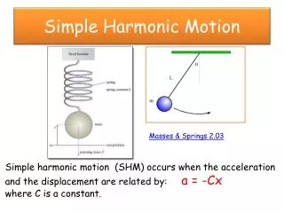
Chapter 13 Simple Harmonic Motion In chapter 13 we will study a special type of motion known as: simple harmonic motion (SHM). It is defined as the motion in which the position coordinate x of an object that moves along the x-axis varies with time t as: x(t) = Asin(t) or x(t) = Acos(t) The condition for having simple harmonic motion is that the force F acting on the moving object is: F = -kx (13-1)
Periodic motion is defined as a motion that repeats itself in time. The period T the time required to complete one repetition Units: s A special case of periodic motion is known as “harmonic” motion. In this type of motion the position x of an object moving on the x-axis is given by: x(t) = Asin(t) or x(t) = Acos(t) The most general expression for x(t) is: The parameters A, , and are constants x(t) = Asin(t + ) (13-2)
Plots of the sine and cosine functions. Make sure that you can draw these two functions /2 = 90º = 180º 3/2 = 270º 2= 360º Note: The period of the sine and cosine function is 2 (13-3)
t m . O x-axis x(t) Most general form of simple harmonic motion x(t) = Asin(t + ) A amplitude angular frequency phase sin(a + b) = (sina)(cosb) +(cosa)(sinb) x = (Acos)sint + (Asin)cost The coordinate x is a superposition of sint and cost functions Special case 1: = 0 x = A sint Special case 1: = /2 x = A cost (13-4)
The effect of the phase on is to shift the Asin(t + ) function with respect to the Asin(t) plot This is shown in the picture below Red curve: Asin(t) Blue curve: Asin(t + ) (13-5)
t m . O x-axis x(t) Determination of A and These two parameters are determined from the initial conditions x(t = 0) and v(t = 0) (13-6)
x = Asin(t) v = Acos(t) Plots of x(t), v(t) and a(t) versus t for = 0 a = -2Asin(t) (13-7)
Consider a point P moving around O on a circular path of radius R win constant angular velocity . The Cartesian coordinates of P are: x and y. The angle = t. From triangle OAP we have: OA = x = Rcost and AP = Rsint The projection of point P on either the x- or the y-axis executes harmonic motion as point P is moving with uniform speed on a circular orbit (13-8) P A
m k x axis O m Fs x axis x A mass m attached to a spring (spring constant k) moves on the floor along the x-axis without friction (13-9)
m k x axis O m Fs x axis x (13-10)
m k x axis O m Fs x axis x (13-11)
m k x axis O m Fs x axis x Summary The spring-mass system obeys the following equation: The most general solution of the equation of motion is: Note 1: The angular frequency ( and thus the frequency f , and the period T) depend on m and k only Note 2:The amplitude A and the phase on the other hand are determined from the initial conditions: x(t = 0) and v(t=0) (13-12) x = Asin(t + )
m k x axis O m Fs x axis x Energy of the simple harmonic oscillator (13-13)
X (13-14)
Why all this fuss about the simple harmonic oscillator? Consider an object of energy E (purple horizontal line) moving in a potential U plotted in the figure using the blue solid line E Motion in the x-axis is allowed in the regions where These regions are color coded green on the x-axis. Motion is forbidden elsewhere (color coded red) If we have only small departures from the equilibrium positions x01 and x02 we can approximate U by the potential of a simple harmonic oscillator (the blue dashed line in the figure) (13-15)
We expand the function U(x) around one of the minima (x01 in this example) using a Taylor series E If we choose the origin to be at xo1 U(x) = kx2/2 This approximation for U is indeed the potential of a simple harmonic oscillator (dotted blue line) (13-16)
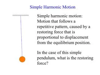
Simple pendulum: A mass m suspended from a string of length that moves under the influence of gravity s (13-17)
Simple Pendulum This differential equation is too difficult to solve. For this reason we consider a simpler version making the “small angle approximation” (13-18)
Summary The simple pendulum (Small angle approximation:) << 1 (13-20)
In the small angle approximation we assumed that << 1 and used the approximation: sin We are now going to decide what is a “small” angle i.e. up to what angle is the approximation reasonably accurate? (degrees) (radians) sin 5 0.087 0.087 10 0.174 0.174 15 0.262 0.259 (1% off) 20 0.349 0.342 (2% off) Conclusion: If we keep < 10 ° we make less that 1 % error (13-21)
O Energy of a simple pendulum C A s = U = 0 B (13-22)
Energy of a simple pendulum (13-23)
O The Physical Pendulum is an object of finite size suspended from a point other than the center of mass (CM) and is allowed to oscillate under the influence of gravity. The torque about point O due to the gravitational force is: r C A d mg (13-24)
O r mg (13-25)
O (13-26) r mg
Fs m x axis x Overall Summary k r (13-27)
Damped Harmonic Oscillator Consider the spring-mass system in which in addition to the spring force Fs = -kx we have a damping force Fd = -bv. The constant b is known as the “damping coefficient” In this example Fd is provided by the liquid in the lower part of the picture -kx v x -bv (13-28)
(13-29) A plot of the solution is given in the figure. The damping force . Results in an exponential decrease of the amplitude with time. The mechanical energy in this case is not conserved. Mechanical energy is converted into heat and escapes.
Fosint Fs m x axis x Driven harmonic oscillator k Consider the spring-mass system that oscillates with angular frequency o = (k/m)1/2 If we drive with a force F(t) = Fosint (where in general o) the spring-mass system will oscillate at the driving angular frequency with an amplitude A() which depends strongly on the driving frequency as shown in the figure to the right. The amplitude has a pronounced maximum when = o This phenomenon is called resonance (13-30)
The effects of resonance can be quite dramatic as these pictures of the Tacoma Narrows bridge taken in 1940 show. Strong winds drove the bridge in oscillatory motion whose amplitude was so large that it destroyed the structure. The bridge was rebuilt with adequate damping that prevents such a catastrophic failure (13-31)