Download

1 / 34
350 likes | 464 Vues
Monty Hall and options. Demonstration: Monty Hall. A prize is behind one of three doors. Contestant chooses one. Host opens a door that is not the chosen door and not the one concealing the prize. (He knows where the prize is.) Contestant is allowed to switch doors. Solution.

E N D
Demonstration: Monty Hall • A prize is behind one of three doors. • Contestant chooses one. • Host opens a door that is not the chosen door and not the one concealing the prize. (He knows where the prize is.) • Contestant is allowed to switch doors.
Solution • The contestant should always switch. • Why? Because the host has information that is revealed by his action.
Representation switch and win or stay and lose guess wrong Nature’s move, plus the contestant’s guess. pr = 2/3 pr = 1/3 guess right switch and lose or stay and win
Definition of a call option • A call option is the right but not the obligation to buy 100 shares of the stock at a stated exercise price on or before a stated expiration date. • The price of the option is not the exercise price.
Example • A share of IBM sells for 75. • The call has an exercise price of 76. • The value of the call seems to be zero. • In fact, it is positive and in one example equal to 2.
S = 80, call = 4 Pr. = .5 S = 70, call = 0 Pr. = .5 t = 1 t = 0 S = 75 Value of call = .5 x 4 = 2
Definition of a put option • A put option is the right but not the obligation to sell 100 shares of the stock at a stated exercise price on or before a stated expiration date. • The price of the option is not the exercise price.
Example • A share of IBM sells for 75. • The put has an exercise price of 76. • The value of the put seems to be 1. • In fact, it is more than 1 and in our example equal to 3.
S = 80, put = 0 Pr. = .5 S = 70, put = 6 Pr. = .5 t = 1 t = 0 S = 75 Value of put = .5 x 6 = 3
Put-call parity • S + P = X*exp(-r(T-t)) + C at any time t. • s + p = X + c at expiration • In the previous examples, interest was zero or T-t was negligible. • Thus S + P=X+C • 75+3=76+2 • If not true, there is a money pump.
Puts and calls as random variables • The exercise price is always X. • s, p, c, are cash values of stock, put, and call, all at expiration. • p = max(X-s,0) • c = max(s-X,0) • They are random variables as viewed from a time t before expiration T. • X is a trivial random variable.
Puts and calls before expiration • S, P, and C are the market values at time t before expiration T. • Xe-r(T-t) is the market value at time t of the exercise money to be paid at T • Traders tend to ignore r(T-t) because it is small relative to the bid-ask spreads.
Put call parity at expiration • Equivalence at expiration (time T) s + p = X + c • Values at time t in caps: S + P = Xe-r(T-t) + C
No arbitrage pricing impliesput call parity in market prices • Put call parity holds at expiration. • It also holds before expiration. • Otherwise, a risk-free arbitrage is available.
Money pump one • If S + P = Xe-r(T-t) + C + e • S and P are overpriced. • Sell short the stock. • Sell the put. • Buy the call. • “Buy” the bond. For instance deposit Xe-r(T-t) in the bank. • The remaining e is profit. • The position is riskless because at expiration s + p = X + c. i.e.,
Money pump two • If S + P + e = Xe-r(T-t) + C • S and P are underpriced. • “Sell” the bond. That is, borrow Xe-r(T-t). • Sell the call. • Buy the stock and the put. • You have + e in immediate arbitrage profit. • The position is riskless because at expiration s + p = X + c. i.e.,
Money pump either way • If the prices persist, do the same thing over and over – a MONEY PUMP. • The existence of the e violates no-arbitrage pricing.
Measuring risk Rocket science
Rate of return = • (price increase + dividend)/purchase price.
Sample versus population • A sample is a series of random draws from a population. • Sample is inferential. For instance the sample average. • Population: model: For instance the probabilities in the problem set.
Population mean • The value to which the sample average tends in a very long time. • Each sample average is an estimate, more or less accurate, of the population mean.
Abstraction of finance • Theory works for the expected values. • In practice one uses sample means.
Explanation • Square deviations to measure both types of risk. • Take square root of variance to get comparable units. • Its still an estimate of true population risk.
Why divide by 3 not 4? • Sample deviations are probably too small … • because the sample average minimizes them. • Correction needed. • Divide by T-1 instead of T.
Derivation of sample average as an estimate of population mean.
Rough interpretation of standard deviation • The usual amount by which returns miss the population mean. • Sample standard deviation is an estimate of that amount. • About 2/3 of observations are within one standard deviation of the mean. • About 95% are within two S.D.’s.
Review question • What is the difference between the population mean and the sample average?
Answer • Take a sample of T observations drawn from the population • The sample average is (sum of the rates)/T • The sample average tends to the population mean as the number of observations T becomes large.