Download
1 / 38
420 likes | 668 Vues
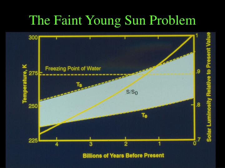
The Faint Young Sun Problem. Systems Notation. = system component. = positive coupling. = negative coupling. Positive Feedback Loops (Destabilizing). Water vapor feedback. Surface temperature. Atmospheric H 2 O. (+). Greenhouse effect. Positive Feedback Loops (Destabilizing).

E N D
Systems Notation = system component = positive coupling = negative coupling
Positive Feedback Loops(Destabilizing) Water vapor feedback Surface temperature Atmospheric H2O (+) Greenhouse effect
Positive Feedback Loops(Destabilizing) Snow/ice albedo feedback Surface temperature Snow and ice cover (+) Planetary albedo
Negative Feedback Loops(Stabilizing) IR flux feedback Surface temperature Outgoing IR flux (-)
Runaway Greenhouse: FIR and FS J. F. Kasting, Icarus (1988)
Negative Feedback Loops(Stabilizing) The carbonate-silicate cycle feedback Rainfall Surface temperature Silicate weathering rate (-) Greenhouse effect Atmospheric CO2
Model pCO2 vs. Time J. F. Kasting, Science (1993)
pCO2 from Paleosols (2.8 Ga) Rye et al., Nature (1995)
Geological O2 Indicators H. D. Holland, 1994
CH4-Climate Feedback Loop Surface temperature CH4 production rate (+) Greenhouse effect
CH4-Climate Feedback Loop • Doubling times for thermophilic methan-ogens are shorter than for mesophiles • Thermophiles will therefore tend to outcompete mesophiles, producing more CH4, and further warming the climate But • If CH4 becomes more abundant than CO2, organic haze begins to form...
Archean Climate Control Loop CH4 production (–) Surface temperature Haze production Atmospheric CH4/CO2 ratio (–) CO2 loss (weathering)
Huronian Supergroup (2.2-2.45 Ga) Redbeds Glaciations Detrital uraninite and pyrite
Snowball Earth Glaciations • Paleomagnetic data indicate low-latitude glaciation at 2.3 Ga, 0.75 Ga, and 0.6 Ga • Huronian glaciation (2.3 Ga) may be triggered by the rise of O2 and the corresponding loss of CH4 • Late Precambrian glaciations studied by Hoffman et al., Science 281, 1342 (1998)
Model pCO2 vs. Time J. F. Kasting, Science (1993)
Late Precambrian Geography *glacial deposits Hyde et al., Nature, 2000
Triggering a Snowball Earth episode • Hoffman et al.: Continental rifting created new shelf area, thereby promoting burial of organic carbon • Marshall et al. (JGR, 1988): Clustering of continents at low latitudes allows silicate weathering to proceed even as the global climate gets cold
Recovering from a Snowball Earth episode • Volcanic CO2 builds up to ~0.1 bar • Ice melts catastrophically (within a few thousand years) • Surface temperatures climb briefly to 50-60oC • CO2 is rapidly removed by silicate weathering, forming cap carbonates
‘Cap’ carbonate (400 m thickness) Hoffman et al., Science, 1998
How did the biota survive the Snowball Earth? • Refugia such as Iceland? • Hyde et al. (Nature, 2000): Tropical oceans were ice free • C. McKay (GRL, 2000): Tropical sea ice may have been thin
Snowball EarthIce Thickness Ts Fg z Toc 0oC Let k = thermal conductivity of ice z = ice thickness T = Toc – Ts Fg = geothermal heat flux
Ice Thickness (cont.) The diffusive heat flux is: Fg = kT / z Solving for z gives: z = kT / Fg 2.5 W/m/K(27 K)/ 6010-3 W/m2 = 1100 m
Heat Flow Through Semi-transparent, Ablating Ice Ref: C. P. McKay, GRL27, 2153 (2000) k dT/dz = S(z) + L + Fg where k = thermal conductivity of ice S(z) = solar flux at depth z in the ice L= latent heat flux (balancing ablation) Fg = geothermal heat flux
Comparative Heat Fluxes Geothermal heat flux: Fg = 6010-3 W/m2 Solar heat flux (surface average): Fs = 1370 W/m2(1 – 0.3)/4 240 W/m2 Equatorial heat flux: Feq 1.2 Fs 300 W/m2 Ratio of equatorial heat flux (from Sun) vs. geothermal heat flux: Feq/Fg 300/0.006 = 5000
Ice Transmissivity C. McKay, GRL (2000)
Heat Fluxes (cont.) Now, let tR = ice transmissivity Then, scaling ice thickness inversely with transmitted heat flux yields: tRz 10-3 ~200 m 10-2 ~20 m 10-1 ~2 m
CONCLUSIONS • Earth’s climate is stabilized on long time-scales by the carbonate-silicate cycle • Higher atmospheric CO2 levels are a good way of compensating for the faint young Sun • CH4 probably made a significant contribution to the greenhouse effect during the Archean when O2 levels were low
CONCLUSIONS (cont.) • Earth’s climate is theoretically susceptible to episodes of global glaciation. It can recover from these by buildup of volcanic CO2 • The first such “Snowball Earth” episode at ~2.4 Ga may have been triggered by the rise of O2 and loss of the methane component of the atmospheric greenhouse
CONCLUSIONS (cont.) • The true “Snowball Earth” model (complete glacial ice cover) best explains the geological evidence, particularly the presence of cap carbonates