Download
1 / 45
470 likes | 640 Vues
Sequence Alignment and Genome Assembly. Zemin Ning The Wellcome Trust Sanger Institute. Outline of the Talk:. Global and Local Alignment Statistical significance of alignment Alignment method. Biological Motivation Why We Need Sequence Alignment. Inference of Homology

E N D
Sequence Alignment and Genome Assembly Zemin Ning The Wellcome Trust Sanger Institute
Outline of the Talk: • Global and Local Alignment • Statistical significance of alignment • Alignment method
Biological Motivation Why We Need Sequence Alignment • Inference of Homology • Two genes are homologous if they share a common evolutionary history. • Evolutionary history can tell us a lot about properties of a given gene • Homology can be inferred from similarity between the genes • Searching for Proteins with same or similar functions
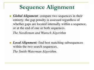
Sequence Alignment Global Alignment: Goal: How similar are two sequences S1 and S2 Input: two sequences S1, S2 over the same alphabet Output: two sequences S’1, S’2 of equal length (S’1, S’2 are S1, S2 with possibly additional gaps) Example: • S1= GCGCATGGATTGAGCGA • S2= TGCGCCATTGATGACC • A possible alignment: S’1=-GCGC-ATGGATTGAGCGA S’2= TGCGCCATTGAT-GACC--
Sequence Alignment (cont) Local Alignment: Goal: Find the pair of substrings in two input sequences which have the highest similarity Input: two sequences S1, S2 over the same alphabet Output: two sequences S’1, S’2 of equal length (S’1, S’2 are substrings of S1, S2 with possibly additional gaps) Example: • S1=GCGCATGGATTGAGCGA • S2=TGCGCCATTGATGACC • A possible alignment: S’1=ATTGA-G S’2= ATTGATG
Global vs. Local Alignment • The Global Alignment Problem tries to find the longest path between vertices (0,0) and (n,m) in the edit graph. • The Local Alignment Problem tries to find the longest path among paths between arbitrary vertices (i,j) and (i’, j’) in the edit graph.
Global vs. Local Alignment (cont’d) • Global Alignment • Local Alignment—betten alignment to find conserved segment --T—-CC-C-AGT—-TATGT-CAGGGGACACG—A-GCATGCAGA-GAC | || | || | | | ||| || | | | | |||| | AATTGCCGCC-GTCGT-T-TTCAG----CA-GTTATG—T-CAGAT--C tccCAGTTATGTCAGgggacacgagcatgcagagac |||||||||||| aattgccgccgtcgttttcagCAGTTATGTCAGatc
Compute a “mini” Global Alignment to get Local Local Alignment: Example Sequence2 Local alignment Global alignment Sequence1
StatisticSignificance of Alignment We need to know how to evaluate the significance of the alignment. There are two scenarios: First, the alignment indicates an evolutionary relationship between the sequences. Second, the alignment is a chance occurrence. What answer is correct? Here, the statistics are important to estimate of probability that the given alignment score might occur by chance.
E Value (E) • E value (E) of an alignment score is the expected number of unrelated sequences in a database that would have a score at least as good. • Low E-values suggest that sequences are homologous. • IfE value ≤ 0.02 sequence probably homologous • IfE value≤ 1 homology cannot be ruled out • IfE value> 1 a match just by chance • Statistical significance depends on both the size of the alignments and the size of the sequence database • Important consideration for comparing results across different searches • E-value increases as database gets bigger • E-value decreases as alignments get longer E value Measuring Alignment Significance
P Value (P) The E-valueis not a probability; it’s an expected value, i.e. the expected outcome. Another criteria of the Alignment Significance is the probability that an alignment with this score could have arisen by chance- p-value: E-value(S) = n • p-value(S), Here n is the number of sequences in the database, S. The lower the p-value, the more likely it is that the alignment score is not by chance but was caused by alignment procedure. For example, p = .01 means there is a 1 in 100 chance the result occurred by chance.
Methods of DNA Sequence Alignment • Dot matrix analysis • The dynamic programming (DP) algorithm • Needleman-Wunsch Algorithm • Smith-Waterman Algorithm • Suffix tree • Hash table based algorithm • Short read alignment tools
Dot Matrix Analysis • A dot matrix analysis is a method for comparing two sequences to look for possible alignment (Gibbs and McIntyre 1970) • One sequence (A) is listed across the top of the matrix and the other (B) is listed down the left side • Starting from the first character in B, one moves across the page keeping in the first row and placing a dot in many column where the character in A is the same • The process is continued until all possible comparisons between A and B are made • Any region of similarity is revealed by a diagonal row of dots • Isolated dots not on diagonal represent random matches
The Needleman-Wunsch Algorithm x = AGTA m = 1 y = ATA s = -1 d = -1 F(i,j) i = 0 1 2 3 4 Optimal Alignment: F(4,3) = 2 AGTA A - TA j = 0 1 2 3
Smith-Waterman Algorithm • Only works effectively when gap penalties are used • In example shown • match = +1 • mismatch = -1/3 • gap = -1+1/3k (k=extent of gap) • Start with all cell values = 0 • Looks in subcolumn and subrow shown and in direct diagonal for a score that is the highest when you take alignment score or gap penalty into account Hij=max{Hi-1, j-1 +s(ai,bj), max{Hi-k,j -Wk}, max{Hi, j-l -Wl}, 0}
Bounded Dynamic Programming Initialization: F(i,0), F(0,j) undefined for i, j > k Iteration: For i = 1…M For j = max(1, i – k)…min(N, i+k) F(i – 1, j – 1)+ s(xi, yj) F(i, j) = max F(i, j – 1) – d, if j > i – k(N) F(i – 1, j) – d, if j < i + k(N) Termination: same Easy to extend to the affine gap case x1 ………………………… xM y1 ………………………… yN k(N)
Suffix Tree Example Mapping the string ababc into a suffix tree. root ab c b abc c abc c
ATGGCGTGCAGTCCATGTTCGGATCA ATGGCGTGCAGT TGGCGTGCAGTC GGCGTGCAGTCC GCGTGCAGTCCA CGTGCAGTCCAT Non-overlap hashing W = N-k+1 (k = 12) ATGGCGTGCAGTCCATGTTCGGATCATTACGTAAGC ATGGGCAGATGT CCATGTTCGGAT CATTACGTAAGC Overlap Hashing W = N/k Non-overlap Hashing v Overlap Hashing
Sequence S: (s1s2, …, si, …, sm) i =1,2, …, m K-tuple: (sisi+1...si+k-1) “A” =00; “C” = 01; “G” = 10; “T” = 11 Sequence Representation Using two binary digits for each base, we may have the following representations: For any of the m/k no-overlapping k-tuples in the sequence, an integer may be used to represent the k-tuple in a unique way where bi = 0 or 1, depending on the value of the sequence base and Emax is the maximum value of the possible E values.
E k-tuple Ni Indices and Offsets 0 AA 1 2, 19 1 AC 3 1, 9 2, 5 2, 11 2 AG 2 1, 15 2, 35 3 AT 2 2, 13 3, 3 4 CA 7 2, 3 2, 9 2, 21 2, 27 2, 33 3, 21 3, 23 5 CC 4 1, 21 2, 31 3, 5 3, 7 6 CG 1 1, 5 7 CT 6 1, 23 2, 39 2, 43 3, 13 3, 15 3, 17 8 GA 4 1, 3 1, 17 2, 15 2, 25 9 GC 0 10 GG 5 1, 25 1, 31 2, 17 2, 29 3, 1 11 GT 6 1, 1 1, 27 1, 29 2, 1 2, 37 3, 19 12 TA 1 3, 25 13 TC 6 1, 7 1, 11 1, 19 2, 23 2, 41 3, 11 14 TG 3 1, 13 2, 7 3, 9 15 TT Hash Table: A 2-tuple hashing table of S1, S2 and S3 S1=(GTGACGTCACTCTGAGGATCCCCTGGGTGTGG) S2=(GTCAACTGCAACATGAGGAACATCGACAGGCCCAAGGTCTTCCT) S3=(GGATCCCCTGTCCTCTCTGTCACATA)
SSAHA seeds Edge length Edge length Sequence for cross_match SSAHA2 = SSAHA + Cross_Match SSAHA for matching seeds, cross_match for sequence alignment.
Read Reference 27 14 25 30 21 29 Mapping Score in ssaha2 • Read mapping score is used to assess the repetitive feature of the read in the genome. With a maximum mapping score 50, we have: • R = read length; Smax - maximum alignment score (smith-waterman) of the hits on genome; Smax2 - second best alignment score of the hits on genome; Say you have one read of 30 bases which has a few hits on the genome: Best hit: exact match with Smax 30; Second best hit: one base mismatch with Smax2 29. The mapping score for this read is Smap = 10;
Genome Assembly using Solexa Short Reads Algorithms and Applications
Outline of the Talk: • Sequence Reconstruction and Euler Path • Assembly strategy • Sequence extension using read pairs, base qualities, fuzzy kmers or longer reads • Repeat junctions • Gap5 - visual inspection for mis-assembly errors
Repeat Repeat Repeat Sequence Repeat Graph Sequences
Sequence Reconstruction - Hamiltonian path approach S=(ATGCAGGTCC) ATG -> TGC -> GCA -> CAG -> AGG -> GGT -> GTC -> TCC ATG AGG TGC TCC GTC GGT GCA CAG • Vertices: k-tuples from the spectrum shown in red (8); • Edges: overlapping k-tuples (7); • Path: visiting all vertices corresponding to the sequence.
CG GT GC AT TG CA GG Sequence Reconstruction - Euler path approach ATG -> TGG -> GGC -> GCG -> CGT -> GTG -> TGC -> GCA ATGCGTGGCA ATGGCGTGCA • Vertices: correspond to (k-I)-tuples (7); • Edges: correspond to k-tuples from the spectrum (8); • Path: visiting all EDGES corresponding to the sequence.
Solexa read assembler to extend short reads to 1-2 kb long reads forward-reverse paired reads known dist ~500 bp 30-75 bp 30-75 bp Capillary reads assembler Phrap/Phusion Genome/Chromosome Assembly Strategy
Pileup of other reads like 454, Sanger etc at a repeat junction Kmer Extension & Repeat Junctions A2 A1 Consensus Means to handle repeats: - Base quality - Read pair - Fuzzy kmers - Closely related reference - 454 or Sanger reads
Handling of Repeat Junctions A = A1 + A2 A2 A1 B1 B = B1 + B2 B2
Handling of Single Base Variations A B1 A B2 B1 = B2 S = A + B1
Salmonella seftenbergSolexa Assembly from Pair-End Reads Solexa reads: Number of reads: 6,000,000;Finished genome size: ~4.8 Mbp; Read length: 2x37 bp; Estimated read coverage: ~92.5 X; Insert size: 170/50-300 bp; Assembly features: - contig stats Solexa 454Total number of contigs: 75; 390 Total bases of contigs: 4.80 Mbp 4.77 Mb N50 contig size: 139,353 25,702 Largest contig: 395,600 62,040 Averaged contig size: 63,969 12,224 Contig coverage on genome: ~99.8 % 99.4% Contig extension errors: 0 Mis-assembly errors: 0 4
maq ssaha2
maq ssaha2
maq ssaha2
maq ssaha2
New Phusion Assembler Assembly Data Process Solexa Reads Supercontig Long Insert Reads PRono Contigs Reads Group Fuzzypath 2x75 or 2x100 Phrap Velvet
Genome Assembly – Normal Cell Solexa reads: Number of reads: 557 Million;Finished genome size: 3.0 GB; Read length: 2x75bp; Estimated read coverage: ~25X; Insert size: 190/50-300 bp; Number of reads clustered: 458 Million Assembly features: - contig statsTotal number of contigs: 1,020,346; Total bases of contigs: 2.713 Gb N50 contig size: 8,344; Largest contig: 107,613 Averaged contig size: 2,659; Contig coverage over the genome: ~90 %; Mis-assembly errors: ?
Acknowledgements: • Jim Mullikin • Yong Gu • Hannes Ponstingl • James Bonfield • Heng Li • Daniel Zerbino (EBI) • Tony Cox • Richard Durbin