Download
1 / 50
500 likes | 612 Vues
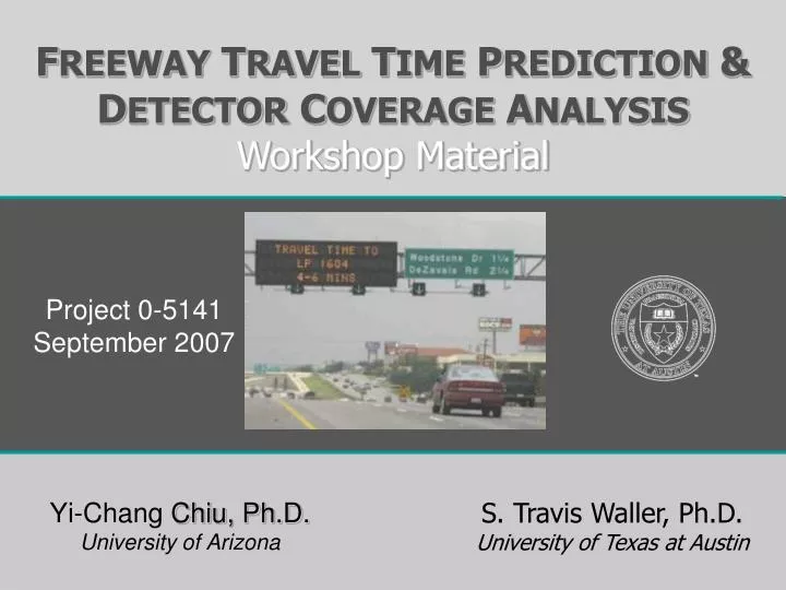
F REEWAY T RAVEL T IME P REDICTION & D ETECTOR C OVERAGE A NALYSIS Workshop Material. Project 0-5141 September 2007. Yi-Chang Chiu, Ph.D. University of Arizona. S. Travis Waller, Ph.D. University of Texas at Austin. Travel Time Classification Summary and conclusions.

E N D
FREEWAY TRAVEL TIME PREDICTION & DETECTOR COVERAGE ANALYSIS Workshop Material Project 0-5141 September 2007 Yi-Chang Chiu, Ph.D. University of Arizona S. Travis Waller, Ph.D. University of Texas at Austin
Travel Time Classification • Summary and conclusions • Introduction • Motivation • Literature Review PART 1: BACKGROUND & TRAFFIC DATABASE Workshop Overview PART 2: INTEGRATED STATISTICAL/SIMULATION MODEL • Concept overview • Software overview • Travel Time Prediction • Detector Placement Analysis • Implementation Issues • Conclusions • Concept overview PART 3: N-CURVE MODEL • Software overview PART 4: TRAFFIC DATABASE GENERATION
PART 1 Introduction
Introduction • Providing freeway travel time prediction • Helps traveling public make pre-trip/en-route travel decision • Increases perceived benefits of ITS infrastructure • Travel time prediction is challenging under non-free-flow situations (e.g. peak hours, incidents, work zones, etc.) due to rapidly changing traffic conditions
Motivation Develop a computationally efficient travel time prediction model Dynamic: reactive to evolving congestion patterns Uses counts from dual loop detectors as inputs (most widely used data collection devices) Develop a model to determine the optimal location of sensors
LiteratureReview State of the Art Short term travel time prediction Time series, regression, Kalman filtering, neural networks, simulation • Conclusions • Many agencies implement naïve estimation methods • Good results under stable/recurrent conditions, but may introduce large errors otherwise • Prediction is necessary to account for multi-segment trips Literature Review State of the practice Travel time estimation speed-based, traffic flow theory Estimate TT Predict TT Prediction Approaches Predict Input Compute TT
A C B D S2 S3 S1 . . 8:00 A.M. 8:05 A.M. 8:10 A.M. Travel Time ClassificationINSTANTANEOUS Travel time on sections at 8:00 A.M tAB(8:00) = tBC(8:00) = tCD(8:00) = 5 min Instantaneous Travel Time (ITT) ITTAD= tAB(8:00) + tBC(8:00) + tCD(8:00) = 15 minutes
A C B D S2 S3 S1 . . 8:00 A.M. 8:05 A.M. 8:10 A.M. Travel Time ClassificationEXPERIENCED & PREDICTED Experienced Travel Time (ETT) ETTAD= tAB(8:00) + tBC(8:00 + tAB(8:00) ) + tCD(8:00 + tAC(8:00)) ETTAD = tAB(8:00) + tBC(8:05) + tCD(8:05+ tBC(8:05)) Notice:ETTAD = ITTAD ONLY if: • tBC(8:05)= 5 minutes • tCD(8:05+ tBC(8:05))=5 minutes Predicted Travel Time (PTT) PTTAD(8:05)= tAB(8:05)+tBC(8:05 + tAB(8:05))+tCD(8:05+ tBC(8:05 + tAB(8:05)) Conditions don’t change
Travel Time ClassificationSUMMARY TRAVEL TIME ESTIMATED • Instantaneous Travel Time • ITT(8:00) =tAB(8:00) + tBC(8:00) + tCD(8:00) • No Prediction/Forecasting Necessary • Experienced Travel Time • ETTAD(8:00)= tAB(8:00)+tBC(8:00+tAB(8:00))+tCD(8:00+tBC(8:00+tAB(8:00))) • Prediction necessary for downstream segments • PREDICTED • PTTAD(8:00)=tAB(8:05)+tBC(8:05+tAB(8:05))+tCD(8:05+tBC(8:05+tAB(8:05))) Prediction necessary for all segments
Lessons Learned • Estimating experienced & predicted travel times is much more difficult than determining instantaneous travel times • Estimation and Prediction involves • Forecasting future conditions on the freeway • Modeling the temporal & spatial evolution of congestion in the freeway section • Implemented models should be able to provide experienced & predicted travel times
PART 2 Integrated Statistical/Simulation Model
MODEL 1Integrated Statistical/Simulation Model STATISTICAL COMPONENT Uses a time series (ARIMA) model to forecast future flows in the on ramps SIMULATION COMPONENT Uses Cell Transmission Model (CTM) to simulate future travel times utilizing forecasted flows
Time Series • Applied in numerous domains to predict future trends from past trends • Time series: sequence of data points collected at uniform time intervals
Time Series Model • Stationary Time Series: Data points vary around a constant mean value • Non-Stationary time series: Exhibit an upward and downward trend • Example: aggregated 5 minute volumes on an on-ramp tend to go up during congestion building phase • Non-Stationary time series can be converted to stationary time series by differencing successive terms
ARIMA Model • Effective for predicting non-stationary time series, like traffic counts • Non-stationary points converted to stationary points by differencing • Instead of using traffic counts at time t as variables (ct), it uses the difference of traffic counts at time t and t-1 (Dct=ct-ct-1) • Differenced stationary points predicted as a function of p past data points and r past errors in prediction • Dct=b+a1x Dct-1+a2xDct-2+…+apxDct-p+Srer
ARIMA Model • Coefficients of the ARMA model are calibrated using past data points. • Most common way is to choose coefficients which minimize the sum of square error between model predictions and actual value in the past data set (More information available in handbook) • Time Series Models are implemented using R, an open source statistical software • The user may easily adjust the time series model specification (p,r) • The source code is flexible, and different statistical components may be used instead of ARIMA models, if desired (such as Kalman filtering)
Cell Transmission Model (CTM) • Mesoscopic Traffic Simulation model developed by Daganzo • Computationally efficient • Captures dynamic traffic phenomena like queue formation, shockwave propagation & link spillovers
A B C Cell Transmission ModelBasic Principles • Freeway segment is converted to cells interconnected by links • Time is discretized in intervals • At each time interval, the model “moves” vehicles from one cell to another, based on traffic flow relationships & cell parameters • Length • Free flow speed • Capacity • Jam Density • Shockwave propagation speed • Travel times are computed based on cumulative counts Calibrated using traffic data
0.4 m 0.5 m 0.6 m 0.3m Origin Cell Gate Cell 23 22 Sink Cell 12 4 3 2 21 7 20 18 1 Merge Cell Sink Cell 24 Cell Transmission ModelConverting the Freeway Segment to Cells • Choose Simulation Interval: Common values between 4 and 10s • Select Free Flow Speed: Estimate the value based on speed limit • Compute Minimum Cell Length: Length > Free Flow Speed * simulation interval • Locate Sensors & Ramps • Divide the segment such that sensors are placed at the beginning of cells, and the minimum cell length is respected • Example: • Free flow speed: 75 mph • Simulation interval: 4sec • Minimum cell length: 440ft • 1st Segment: 4 cells of 528 • 3st Segment: 6 cells of 452 ft • + 1 cell of 456ft • 4st Segment: 3 cells of 528
MODEL 1Software • A single software tool can be used for: • CTM parameter calibration • Travel time prediction • Detector location
Software Installation • Install R – open source statistical software available for free from http://cran.cnr.berkeley.edu/ • Create a Working Folder • Copy files R-Arima.txt,original code.exe original code.exe.config into the working folder • Adjust path information in R-Arima.txt to reflect path of working folder
Calibration Process Run model with estimated values for the input parameters Compare model outputs with calibration data NO Adjust parameters Desired accuracy? YES Calibration Completed
Calibration Mode • Parameters to be calibrated • Jam Density • Maximum Flow (Capacity) • Speed of Backward Moving Shockwave • Free Flow Speed • Calibration options: • Based on travel times (only possible if real travel time measurements are available): minimize the difference between ctual section travel time travel time and travel time predicted by model (read from output.txt) • Based on cumulative counts at sensor locations (always feasible): minimize the difference between cumulative counts at each sensor and counts predicted by the model (read from volumes-calibration.txt) • The software documentation provides further information about the calibration procedure
Online Travel Time PredictionInput Data NETWORK DATA INPUT DATA LINK DATA REAL TIME TRAFFIC DATA GUI • Adjustments to the source code are necessary to adapt the model to the TMC operations characteristics (such as frequency of data provision & travel time computations, desired aggregation) • Historical data can be used to test the model performance • The model will read only a specified number of data points at the time, and therefore behave as if it was actually working in real time • The software documentation provides detailed explanations
Online Travel Time PredictionProcedure • Prepare Input Files • Convert the freeway segment into cells • Select & Calibrate Parameters • Adjust TMC preferences (such as frequency of predictions) • Execute the model • Analyze output files • Travel time predictions per OD pair, at desired intervals and aggregation levels • Adjust model options based on performance
Offline Detector Coverage AnalysisBasic Algorithm & Options Generate one possible detector deployment pattern or read it from the input file Example of possible patterns for 3 sensors Compute travel time prediction error • Model options • Automatically generate ALL possible patterns • A threshold for the minimum distance between detectors may be included to reduce the umber of feasible patterns • Feed a set of patterns manually Are there other possible patterns ? YES NO Analyze Errors and select optimal location
Offline Detector Coverage AnalysisSome Considerations • Additional Input data (described in detail in the documentation) • Relative position of cells (if deployment patterns are generated automatically) • Possible deployment patterns (if only a set of possible patterns is analyzed) • Real travel times for all the analyzed OD pairs • Real sensor counts are needed for all possible sensor locations • Data should be generated using a microscopic traffic simulator, such as VISSIM • Output files provide several error measurements for all the analyzed patterns • Global error measurements are indicative of the convenience of a deployment strategy • Selecting an optimal pattern is not straightforward, some patterns may lead to lower global error, but favor the performance for certain OD pairs • Final decision is based on engineering judgment • Specific criteria can be incorporated in the source code
General Software Features & Implementation Issues • Runs on a standard PC • Relies on count data, easily obtainable using loop detectors • As with any model, model performance will vary depending on accuracy of data • Additional layer of data screening and filtering should be incorporated to ensure accurate results • Characteristics of the layer are TMC specific • Objectives include (more information in the final report): • Generate input data files compatible with the model in terms of file names, aggregation levels, frequency of updates, etc • Identify malfunctioning sensors • Exclude them from the simulation • Use some procedure to impute the missing data • Identify extreme traffic conditions which demand for manual adjustment of model parameters
Conclusions • Travel time prediction is desirable to help drivers to make informed decisions • Naïve prediction procedures are not accurate enough during unstable traffic conditions • The model developed for this project has the potential to improve upon existing methodologies • Final adjustment for real-time operation are TMC specific, and need to be accomplished before deployment • Model performance should be monitored, and modifications to the following components may be used to improve results • Heuristic procedure to re-set initial densities (explained in the final report) • Statistical component • Data filtering layer • The detector coverage analysis tool provided with this package is useful to evaluate potential detector locations, and consider re-location of existing sensors • CTM is a powerful methodology to model traffic flows. The software provided for this project can be used to develop and calibrate CTM models for other purposes
PART 3 N Curve Model
Problems Statement • On a basic freeway segment, given a set of detectors, which are able to provide traffic counts at a fixed frequency, • the problem is to provide predicted experience travel time at any time t from a pre-defined DMS location to a pre-defined prediction target destination at each pre-defined update instance over the pre-defined operational horizon.
Problems Statement (cont’d) • Given #1: • Number and locations of detectors • Historical data for each detector (distribution information) • DMS and prediction target destination location • Notations: • distance between detector d1 and d2, • experienced travel time from d1 to d2 predicted at time t, • cumulative traffic counts at detector #1 at time t, • cumulative traffic counts at detector #2 at time t, • Property 1 • d1 is upstream of d2 Where • Property 2 • Note: no over-taking is considered • Question to be asked, how do we determine the following: where and
Given #2 . . Notations: mean of vehicle(s) n at sensor i at time t, standard deviation of vehicle(s) n at sensor i at time t, mean of time t at sensor i for vehicle(s) n, standard deviation of time t at sensor i for vehicle(s) n, cumulative traffic counts at detector i at time tp, cumulative traffic counts at detector j at time tp, Problems Statement (cont’d)
Problems Statement (cont’d) • Property 1 • Model at time tp (time instance at which prediction is needed) • DMS location i • Prediction target destination j • Question to be asked, how do we find t* such that: • Model 1 • Find t* such that of Predicted travel time interval of • Predicted travel time interval
PART 4 Traffic Database Generation
Traffic Database • Contains detector fromTransVISTA • 77 detectors • 37 miles (11 on El Paso Border Highway) • An online graphic user interface (GUI) is provided to access sensor data • Complemented w/some real travel time measurements obtained via GPS
Traffic Database ONLINE GUI
Daily TAR file • Sender program • PcAnywhere Remote Modem Daily TAR file Receiver program PcAnywhere Host TCPIP - JDBC URL Connection to Postgres server TxDoT GUI hosted by U of A TTI TTI Database U of A Database Data Transfer Schematic • Major nodes • TxDOT • TTI • U of A
Record 1 Record 2 Record 3 . . . . Database: FTMS File • Hex file template
Database Objects • Each of this objects will be populated with data read from the hex file • Examples • Sensor ID • Time (hour, minute and second) • Date (day, month and year) • Volume, speed and occupancy
Problems Encountered • Modem communication • Unreliable nature of modem communication • Unreliable data transfer • Difficulty in running programs together • Must stop program transfers to address difficulties • When modems do not respond… • Manual intervention at both TxDOT and TTI is required • Programs must be stopped to address difficulties
Problems Encountered (cont’d) • Midnight transfer • Reading of new file at TxDoT • Data from TTI has to be inserted into a new table. • This switch has been tested but a period of no data for several hours after midnight has been detected. • The problem has been resolved as of last visit to TransVista