Download
1 / 1
10 likes | 129 Vues
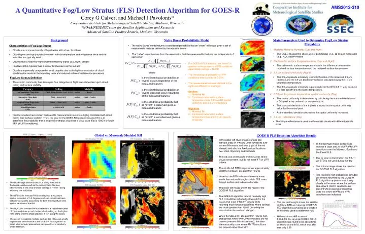
AMS2012-310. A Quantitative Fog /Low Stratus (FLS) Detection Algorithm for GOES-R Corey G Calvert and Michael J Pavolonis* Cooperative Institute for Meteorological Satellite Studies, Madison, Wisconsin *NOAA/NESDIS/Center for Satellite Applications and Research

E N D
AMS2012-310 A Quantitative Fog/Low Stratus (FLS) Detection Algorithm for GOES-R Corey G Calvert and Michael J Pavolonis* Cooperative Institute for Meteorological Satellite Studies, Madison, Wisconsin *NOAA/NESDIS/Center for Satellite Applications and Research Advanced Satellite Product Branch, Madison Wisconsin Background Naïve Bayes Probabilistic Model Main Parameters Used to Determine Fog/Low Stratus Probability Characteristics of Fog/Low Stratus • Clouds are composed mainly of liquid water with a low cloud base • Cloud layers are highly spatially uniform in both temperature and reflectance since vertical velocities are typically weak • Clouds have a relatively high spectral emissivity signal (3.9,11m) at night • Fog/low stratus typically has a similar temperature as the surface • Clouds are generally composed of small droplets due to the high concentration of cloud condensation nuclei in the boundary layer and reduced collision/coalescence processes • Fog/Low Stratus Definition • The aviation community has developed four categories of flight rules dependent upon cloud ceiling and surface visibility. • Previous studies have shown that satellite measurements are more highly correlated with cloud ceiling than surface visibility. Thus, the goal for the GOES-R fog detection algorithm is to determine the probability that a single-layer stratus cloud has a cloud base that is 1000 ft or lower (IFR or LIFR conditions). • The naïve Bayes’ model returns a conditional probability that an “event” will occur given a set of measureable features defined by the equation below • The “naïve” aspect comes from the assumption that the measureable features are independent of each other • Modeled Relative Humidity (Day and Night) • The GOES-R algorithm allows use of both Global (e.g., GFS) and mesoscale(e.g., RUC) NWP models • Radiometric surface temperature bias (Day and Night) • The radiometric surface temperature bias is the difference between the modeled surface temperature and the retrieved surface temperature. • 3.9 μm pseudo-emissivity (Night) • The 3.9 m pseudo-emissivity is simply the ratio of the observed 3.9 m radiance and the 3.9 m blackbody radiance calculated using the 11 m brightness temperature. • The 3.9 m pseudo-emissivity is preferred over the BTD(3.9-11 m) because it is less sensitive to the scene temperature. • 0.65 μm brightness temperature spatial uniformity (Day) • The spatial uniformity is determined by calculating the standard deviation of a 3x3 pixel array centered on any given pixel. • The standard deviation of the 9 pixels is stored as the spatial uniformity value for the central pixel. • As the standard deviation decreases the spatial uniformity increases. • 3.9 μm reflectance (Day) • The 3.9 m reflectance is used to differentiate clouds with different particle sizes • For GOES-R FLS detection the “event” in question is the presence of IFR conditions (specifically ceilings < 1000ft) • The climatological probability of IFR conditions was found to be 9.73% • The measureable features (defined to the right) are different for day/night: • Daytime • Modeled RH • Combined radiometric surface temperature bias, 0.65 m BT spatial uniformity and 3.9 m reflectance • Nighttime • Modeled RH • Combined radiometric surface temperature bias and 3.9 m pseudo-emissivity where is the climatological probability an “event” occurs regardless of the measured features is the climatological probability an “event” does not occur regardless of the measured features Is the conditional probability that an “event” is observed given a measured feature Is the conditional probability that an “event” is not observed given a measured feature Global vs. Mesoscale Modeled RH GOES-R FLS Detection Algorithm Results • In the upper left RGB image, surface obs indicate areas of IFR and LIFR conditions over eastern Minnesota and Iowa (right of the red triangle) and also in a few localized locations over Utah, Wyoming and Colorado • The red oval and triangle enclose areas where clouds are present, but do not meet IFR or LIFR criteria • The middle left BTD image shows approximately what the heritage FLS algorithm returns • Note that the BTD indicates the entire areas inside the oval and triangle contain FLS, even though surface obs indicate otherwise • The lower left image shows the result of the GOES-R FLS algorithm • The GOES-R algorithm returns relatively high FLS probabilities (shaded yellow-red) for the clouds that meet IFR/LIFR criteria while returning much lower probabilities where ceilings are much greater than 1000ft (including the areas inside the oval and triangle) • When the GOES-R FLS algorithm returns high probabilities where IFR/LIFR conditions are not present (western Minnesota/Iowa), the false alarms usually occur where MVFR conditions are present rather than VFR • In the top RGB image, surface obs indicate a large area of MVFR/IFR/LIFR conditions over the Midwest, South and Southeast U.S. • Due to solar contamination the 3.9–11 m BTD is not used during the day • The bottom image shows the result of the GOES-R FLS algorithm • The relatively high probabilities (shaded yellow-red) returned by the GOES-R FLS algorithm appear to match very closely to the areas where the surface obs show IFR/LIFR conditions are present while keeping probabilities quite low where MVFR and VFR conditions are indicated • The RGB image above shows FLS along the Central California coast as well as the valley inland. Surface observations in the area showed ceilings of ~100 f t along with very low visibilities • The GFS 12-hr forecast RH is available at a maximum spatial resolution of 0.5 degrees and can sometimes have difficulty accurately accounting for both the magnitude and spatial variation of the RH • The RUC 2-hr forecast RH is available at a spatial resolution of 13km and does a much better job of picking up the higher RH’s along with the sharp gradient in RH along the coast. • The use of mesoscale models, such as the RUC, can greatly improve the performance of the GOES-R FLS algorithm in areas where model parameters vary greatly over relatively small distances • The plot on the right shows the skill the nighttime BTD and day/night GOES-R FLS algorithms achieved as a function of threshold used to determine FLS • With maximum skill scores of 0.70/0.59, the day/night GOES-R FLS algorithm was found to be about twice as skillful as the BTD, which max skill was only 0.28