Download

1 / 58
580 likes | 582 Vues
This paper presents a region labeling approach to automatically locate and extract moving objects from video sequences. The proposed algorithm includes global motion estimation, initial partition, watershed segmentation, spatio-temporal merge, and initial classification. The method is accurate and robust, providing efficient and precise segmentation results.

E N D
Automatic Segmentation of Moving Objects in Video Sequences: A Region Labeling Approach Amir Averbuch Yaki Tsaig School of Computer Science Tel Aviv University Tel Aviv, Israel
Problem Statement • We wish to locate and extract moving objects (VOPs) from a sequence of color images, to be used for content-based functionalities in MPEG-4
Original frame Initial partition Motion estimation Final segmentation Classification The Suggested Approach
Global Motion Estimation • The camera motion is modeled by a perspective motion model • This model assumes that the background can be approximated by a planar surface. • The estimation is carried out using a robust, gradient-based technique, embedded in a hierarchical framework.
Motion-compensated differences Raw differences Global Motion Estimation & Compensation – Example
Initial Partition An initial spatial partition of each frame is obtained by applying the following steps: • Color-based gradient approximation • Watershed segmentation • Spatio-temporal merge
Initial Partition - Goals • Each region in the initial partition should be a part of a moving object or part of the background. • The number of regions should be low (100-300), to allow an efficient implementation. • Regions should be big enough to allow a robust motion estimation.
Gradient Approximation • The spatial gradient is estimated using Canny’s gradient approximation. • Specifically, Canny’s gradient is computed for each of the three color components Y, Cr and Cb, by convolving each color component with the first derivative of a Gaussian function. • A common gradient image is generated by
Watershed Segmentation • An initial partition is obtained by applying a morphological tool known as watershed segmentation, which treats the gradient image as a topographic surface. • The surface is flooded with water, and dams are erected where the water overflows
Watershed Segmentation (2) Rain-falling Implementation • Each drop of water flows down the steepest descent path, until it reaches a minimum. • A drowning phase eliminates weak edges by flooding the surface with water at a certain level
Original image Watershed segmentation Watershed Segmentation (3)
Watershed Segmentation (4) Advantages: • The resulting segmentation is very accurate – the watersheds match the object boundaries precisely • The rain-falling implementation is significantly faster than any other segmentation technique Disadvantages: • The technique is extremely sensitive to gradient noise, and usually results in oversegmentation
Spatio-Temporal Merge • In order to eliminate the oversegmentation caused by the watershed algorithm, a post-processing step is employed, that eliminates small regions by merging them. • To maintain the accuracy of the segmentation, temporal information is considered in the merge process.
Spatio-Temporal Merge (2) Spatial Distance: Temporal Distance:
Spatio-Temporal Merge (3) • Set Tsz = 20 • For each region Riwhose size is smaller than Tsz, merge it with its neighbor Rjwhich satisfies Tsz = Tsz + 20 If Tsz > 100, stop. Otherwise, go back to II.
Spatio-Temporal Merge (4) Iterations: 1 , 2 , 3 , 4 , 5
Initial Classification • The initial classification phase marks regions as potential foreground candidates, based on a significance test • It serves two purposes: • It reduces the computational load of the classification process. • It increases the robustness of the motion estimation, by eliminating noisy background regions.
Initial Classification (2) • We assume that the sequence is subject to camera noise, modeled as additive white Gaussian noise (AWGN) • Under the assumption that no change occurred (H0), the differences between successive frames are due to camera noise
Initial Classification (3) • To increase the robustness of the test, a local sum is evaluated • The local sum follows a chi-squared distribution, thus a threshold can be computed by specifying a significance level, according to
Initial Classification (4) • For each region in the initial partition: • If the majority of the pixels within the region appear in the tracked mask of the previous frame, mark this region as a foreground candidate • Otherwise, compute the local sum Δk for each pixel in the region, and apply the significance test • If the number of changed pixels in the regions exceeds 10% of the total number of pixels, mark this region as a foreground candidate, otherwise mark it as background
Original frame Changed areas Initial classification Reference frame Initial Classification (5)
Motion Estimation • Following the initial classification phase, the motion of potential foreground candidates is estimated • The motion estimation is carried out by hierarchical region matching • The search begins at the coarsest level of the multi-resolution pyramid • The best match at each level is propagated to the next level of the hierarchy, and the motion parameters are refined
Motion Estimation (2) Advantages: • Region-based motion estimation does not suffer from the local aperture problem • Since the initial partition is usually accurate, motion discontinuities are handled gracefully Disadvantages: • Like most motion estimation techniques, this method suffers from the occlusion problem
Frame #21 Frame #24 Motion field Moving regions Motion Estimation (3)
Motion Validation • Let us assume that the estimated motion satisfies the brightness change constraint, • If the motion vector is valid, then the differences dk in the occlusion area satisfy where n is a zero-mean Gaussian noise
Motion Validation (2) • Conversely, if the motion vector is invalid, then the differences inside the occlusion area are attributed only to camera noise • Therefore, we can define the two hypotheses as
Motion Validation (3) • Equivalently, we can write • Using the Maximum Likelihood criterion, we obtain
Motion Validation (4) • For each region, apply the decision rule on the pixels within the occlusion area. The decision for the entire region is based on the majority • If the estimated motion vector is invalid, mark the occlusion area and perform the hierarchical motion estimation again, while considering only displacement • Repeat the last step iteratively, until the motion of the region is valid
Frame #21 Frame #24 Before validation After validation Motion Validation (5)
Classification Using a Markov Random Field Model • In order to classify each of the regions in the initial partition as foreground or background, we define a Markov random field(MRF) model over the region adjacency graph (RAG) constructed in the initial partition phase.
Classification Using a Markov Random Field Model (2) • To obtain a classification of the regions in the RAG, we need to find a configuration ωof the MRF X, based on an observed set of features O, such that the a-posteriori probability P(X=ω|O) is maximal. • Using Bayes’ rule and Hammersley-Clifford theorem, it can be shown that the a-posteriori probability of the MRF follows a Gibbs distribution
Classification Using a Markov Random Field Model (3) • Thus, the optimal configuration of the MRF (minimal probability of error estimate) is obtained using • Therefore, a classification of the regions is achieved by minimizing the energy function Up(ω|O)
The MRF Model • To define the MRF model, we use the following notations: • A label set L = {F,B}, where F denotes foreground and B denotes background. • A set of observations O = {O1,…,ON}, where Oi = {MVi,AVGi,MEMi}, and • MVi is the estimated motion vector for the region • AVGi is the average intensity value inside the region • MEMi is the memory value inside the region
The MRF Model (2) • We define the energy function of the MRF as Motion Temporal continuity Spatial continuity
The MRF Model (3) • ViM is the motion term, which represents the likelihood of region Rito be classified as foreground or background, based on its estimated motion
The MRF Model (4) • ViT is the temporal continuity term, which allows us to consider the segmentation of prior frames in the sequence, and maintain the coherency of the segmentation through time
The MRF Model (5) • VijS is the spatial continuity term, which imposes a constraint on the labeling, based on the spatial properties of the regions • The similarity function f(·) is given by
Optimization Using HCF • The optimization of the energy function of the MRF model is performed using Highest Confidence First (HCF) • The nodes of the graph are traversed in order of their stability • In each iteration, the label of the least stable node is changed, so that the decrease in its energy is maximal, and its neighbors are updated accordingly
MRF Labeling – Example Original frame Initial partition Initial classification 160 Regions 100 Regions 174 Regions 140 Regions 120 Regions 40 Regions 60 Regions 80 Regions 20 Regions 0 Regions Final segmentation MRF labeling Motion estimation
Object Tracking & Memory Update • In order to maintain temporal coherency of the segmentation, a dynamic memory is incorporated • The memory is updated by tracking each foreground region to the next frame, according to its estimated motion vector • Infinite error propagation is avoided by slowly decreasing memory values of background regions
Frame #21 Frame #19 Frame #23 Frame #25 Frame #13 Frame #3 Frame #11 Frame #7 Frame #15 Frame #5 Frame #17 Frame #27 Frame #29 Frame #31 Frame #41 Frame #45 Frame #35 Frame #1 Frame #9 Frame #33 Frame #43 Frame #39 Frame #37 Object Tracking & Memory Update (2)
Experimental Results Mother & Daughter Initial partition Initial classification Original frame Motion estimation MRF labeling Extracted VOP
Frame #55 Frame #91 Frame #127 Experimental Results (2) Mother & Daughter
Experimental Results (3) Miss America Initial partition Initial classification Original frame Motion estimation MRF labeling Extracted VOP
Frame #11 Frame #39 Frame #24 Experimental Results (4) Miss America
Experimental Results (5) Silent Initial partition Initial classification Original frame Motion estimation MRF labeling Extracted VOP
Frame #55 Frame #118 Frame #91 Experimental Results (6) Silent
Experimental Results (7) Foreman Initial partition Initial classification Original frame Motion estimation MRF labeling Extracted VOP