Download
1 / 20
200 likes | 377 Vues
Standardizing catch per unit effort data. Standardization of CPUE. Catch = catchability * Effort * Biomass CPUE = Catch/Effort = U = catchability * Biomass U t = qB t U t : Catch per unit effort at time t q : catchability of the whole fleet

E N D
Standardization of CPUE • Catch = catchability * Effort * Biomass • CPUE = Catch/Effort = U = catchability * Biomass • Ut = qBt • Ut: Catch per unit effort at time t • q : catchability of the whole fleet • catchability: the proportion of the stock caught per one unit of effort • In most fisheries we normally have fleets with different catchabilities • Lets start by looking at a fishery on a stock where we have vessel types (i) that have different catchabilities: • Ut,i: Catch per unit effort of vessel type i at time t • qi : catchability of vessel type i
A very simplified artificial case: 2 Fleets • For illustration we create some CPUE data for 6 years for 2 fleets from known stock size, effort and catchability • Catchability is fleet specific, with fleet 2 having 3 times higher catchability than fleet 1 • Effort in Fleet 1 declines while it increases in fleet 2. Total effort remains constant
Relative values • lets standardize the overall CPUE series relative to that of the first year: • it is obvious that ignoring the different catchabilities of fleet 1 and 2 would lead wrong conclusion about biomass development • however, if we were to use either Fleet 1 OR 2 we would get accurate representation of the relative change in biomass • CPUE from some “selected” fleet, which is assumed to be homogenous over time is often used in practice • The problem is that the assumption of homogeneity is an assumption in real cases!
Relative stock size and overall CPUE it is obvious that ignoring the different catchabilities of fleet 1 and 2 would lead wrong conclusion about biomass development when using the
Standardizing the catch rate of each fleet • lets standardized the CPUE series of each fleet relative to the first year: • if we were to use either Fleet 1 OR 2 we would get accurate representation of the relative change in biomass • CPUE from some “selected” fleet, which is assumed to be homogenous over time are often used in practice
General linear modeling of CPUE data – the math • Relative changes in biomass: • Lets first describe changes in biomass relative to the first year in the data series: • Bt – biomass at time t • B1 – biomass in year 1 • at – scaling factor • where: • and hence a1 = 1.00 The aim is to use the at parameter in the relationship Ut = qBt
General linear modeling of CPUE data – the math • We have • then • the a92, a93, a94, … are hence (again) a measure of biomass (B) relative to a91 = 1.00 but here we have related it to CPUE • more importantly we gotten rid of the actual biomass (B)!
General linear modeling of CPUE data – the math • The relationship: • only applies to homogenous fleet • Lets revisit the imaginary 2 vessel class fisheries (where we “know” that q within a fleet has remained constant): • Here the b2|1 is the efficiency of vessel class 2 relative to vessel class 1. • The mathematical formula is effectively saying: • the CPUE of vessel class 2 at any one time t is just a multiplier of CPUE of vessel class 1 at time t taking into account changes relative changes in biomass (at) since first year
General linear modeling of CPUE data (4) • In general for multivessel fisheries we can write • where • i: vessel size class i • Ut,i : CPUE of the for time t and vessel class i • U1,1: CPUE of the 1st vessel class in the 1st time period • bi: The efficiency of vessel class i relative to vessel class 1 • at: Relative abundance • Food for thought: • What is the value of at when t = 1? • What is the value of bi when i = 1?
General linear modeling of CPUE data (5) • To take into account measurement errors the statistical model becomes: • The error can be normalized by transformation: • We hence have a general linear model which can be used to estimate the parameters. For stock assessment purposed the parameters at is of most interest. However, one could consider that the bi parameters may be of interest in terms of understanding the fishery and for management • What we have here is nothing more than: Yi = Ŷi + i • … and we know how we estimates the parameters of such a simple model • Food for thought: • What is the value of ln(at) when t = 1? • What is the value of ln(bi) when i = 1?
General linear modeling of CPUE data (6) • The GLIM model fit is often done by rescaling all the cpue observation to that of U1,1 (as we have already done) I.e.:
Our example • Lets first add some measurement noise (stochasticity) to our artificial deterministic CPUE data:
Spreadsheet schematics of the model for the simplified example • The ln-value for t=1 and i=1 is by definition zero • The b value for the reference fleet i=1 is always zero, irrespective of the year (t) • The a value for the reference fleet i=2 is the same as for i=1 within each year Just moving the parameter values here for clarity/convenience
Best fit Minimized the squared residuals to obtain the best parameter estimates
Expanding the GLM model • The expansion of the GLM model to take into account: • Area • Season/month • … • is mathematically straightforward: • the model fitting process is the same?
Where it goes wrong … • Catch rate may not be proportional to abundance • Hence the abundance trend from GLM will not be proportional to abundance • Any changes unrelated to quantifiable effects will not be captured in the GLM analysis. • In such cases the change will wrongly be ascribed to changes in abundance • e.g. increase in vessel efficiency within a fleet class due to increased skill • ERGO: • GLM analysis is the best tool available to calculate standardized catch rate • Weather the actual abundance trend form GLM represents true changes in stock abundance will always be a subjective call