Download
1 / 71
710 likes | 722 Vues
Data Structures – Week # 10. Graphs & Graph Algorithms. Outline. Motivation for Graphs Definitions Representation of Graphs Topological Sort Breadth-First Search (BFS) Depth-First Search (DFS) Single-Source Shortest Path Problem (SSSP) Dijkstra’s Algorithm Minimum Spanning Trees

E N D
Data Structures – Week #10 Graphs & Graph Algorithms
Outline • Motivation for Graphs • Definitions • Representation of Graphs • Topological Sort • Breadth-First Search (BFS) • Depth-First Search (DFS) • Single-Source Shortest Path Problem (SSSP) • Dijkstra’s Algorithm • Minimum Spanning Trees • Prim’s Algorithm • Kruskal’s Algorithm Borahan Tümer, Ph.D.
Graphs & Graph Algorithms Borahan Tümer, Ph.D.
Motivation • Graphs are useful structures for solving many problems computer science is interested in including but not limited to • Computer and telephony networks • Game theory • Implementation ofautomata Borahan Tümer, Ph.D.
Graph Definitions • A graphG=(V,E) consists a set of verticesV and a set of edgesE. • An edge(v,w)E has a starting vertex v and and ending vertex w. An edge sometimes is called an arc. • If the pair is ordered, then the graph is directed. Directed graphs are also called digraphs. • Graphs which have a third component called a weight or costassociated with each edge are called weighted graphs. Borahan Tümer, Ph.D.
Adjacency Set and Being Adjacent • Vertex v is adjacent to u iff (u,v)E. In an undirected graph with e=(u,v), u and v are adjacent to each other. • In Fig. 6.1, the vertices v, w and x form the adjacency set of u or Adj(u)={v,w,x}. u v w x Figure 6.1. Adjacency set of u Borahan Tümer, Ph.D.
More Definitions • A cycle is a path such that the vertex at the destination of the last edge is the source of the first edge. • A digraph is acycliciff it has no cycles in it. • In-degree of a vertex is the number of edges arriving at that vertex. • Out-degree of a vertex is the number of edges leaving that vertex. Borahan Tümer, Ph.D.
Path Definitions • A path in a graph is a sequence of vertices w1, w2, …,wn where each edge (wi, wi+1)E for 1i<n. • The length of a path is the number of edges on the path, (i.e., n-1 for the above path). A path from a vertex to itself, containing no edges has a length 0. • An edge (v,v) is called a loop. • A simplepath is one in which all vertices, except possibly the first and the last, are distinct. Borahan Tümer, Ph.D.
Connectedness An undirected graph is connected if there exists a path from every vertex to every other vertex. • A digraph with the same property is called strongly connected. • If a digraph is not strongly connected, but the underlying graph (i.e., the undirected graph with the same topology) is connected, then the digraph is said to be weakly connected. • A graph is complete if there is an edge between every pair of vertices. Borahan Tümer, Ph.D.
Representation of Graphs • Two ways to represent graphs: • Adjacency matrix representation • Adjacency list representation Borahan Tümer, Ph.D.
Adjacency Matrix Representation • Assume you have n vertices. • In a boolean array with n2 elements, where each element represents the connection of a pair of vertices, you assign true to those elements that are connected by an edge and false to others. • Good for densegraphs! • Not very efficient for sparse (i.e., not dense) graphs. • Space requirement: O(|V|2). Borahan Tümer, Ph.D.
Adjacency matrix representation (AMR) 5 7 1 2 3 6 7 4 9 8 3 4 4 5 6 8 6 3 7 9 5 3 7 8 9 4 1 3 6 Disadvantage: Waste of space for sparse graphs Advantage: Fast access Borahan Tümer, Ph.D.
Adjacency List Representation Assume you have n vertices. • We employ an array with n elements, where ith element represents vertex i in the graph. Hence, element i is a header to a list of vertices adjacent to the vertex i. • Good for sparse graphs • Space requirement:O(|E|+|V|). Borahan Tümer, Ph.D.
5 7 1 2 3 1 2,7 4,8 5,9 8,3 6 7 2 3,5 6,4 7,9 9,3 4 9 8 3 4 3 4,6 4 5 6 4 9,5 8 6 5 2,4 3,7 6,8 7,3 8,6 3 7 9 5 3 6 9,7 7 8 9 7 8,4 9,6 4 1 3 8 9,1 9 9,3 Adjacency list representation (ALR) array index: source vertex; first number: destination vertex; second number: cost of the corresponding edge 6 Disadvantage: Sequential search among edges of a node Advantage: Minimum space requirement Borahan Tümer, Ph.D.
Topological Sort • Topological sort is an ordering of vertices in an acyclic digraph such that if there is a path from vi to vj, then vj appears after vi in the ordering. • Example: course prerequisite requirements. Borahan Tümer, Ph.D.
Algorithm for Topological Sort* Void Toposort () { Queue Q; int ctr=0; Vertex v,w; Q=createQueue(NumVertex); for each vertex v if (indegree[v] == 0) enqueue(v,Q); while (!IsEmpty(Q)) { v=dequeue(Q); topnum[v]=++ctr; for each w adjacent to v if (--indegree[w] == 0) enqueue(w,Q); } if (ctr != NumVertex) report error (‘graph cyclic!’) free queue; } *From [2] Borahan Tümer, Ph.D.
s t r w u v r x z y Q TN An Example to Topological Sort Q is indicated by the red squares. TN keeps track of the order in which the vertices are processed. Borahan Tümer, Ph.D.
s t r u w v r v v r 0 0 x z y Q TN An Example to Topological Sort Borahan Tümer, Ph.D.
s t r u w v r s x v 1 0 x z y Q TN An Example to Topological Sort Borahan Tümer, Ph.D.
s t r u w v x r v s 1 2 0 x z y Q TN t w An Example to Topological Sort Borahan Tümer, Ph.D.
r s v x 2 3 0 1 An Example to Topological Sort s t r u w v x z y y t w Q TN Borahan Tümer, Ph.D.
s v r x 0 2 1 3 An Example to Topological Sort s t r u w v x z y y u t w Q TN 4 Borahan Tümer, Ph.D.
s v r x 0 2 1 3 An Example to Topological Sort s t r u w v x z y y u t w Q TN 4 5 Borahan Tümer, Ph.D.
s t r u w v s r x v 2 3 0 1 x z y Q TN y u t w 6 4 5 An Example to Topological Sort Borahan Tümer, Ph.D.
z x s v r 3 2 0 1 An Example to Topological Sort s t r u w v x z y y u t w Q TN 6 7 4 5 Borahan Tümer, Ph.D.
s t r u w v x s r z v 0 2 8 1 3 x z y y u t w Q TN 6 7 4 5 An Example to Topological Sort Borahan Tümer, Ph.D.
Breadth-First Search (BFS) • Given a graph, G, and a source vertex, s, breadth-first search (BFS) checks to discover every vertex reachable from s. • BFS discovers vertices reachable from s in a breadth-first manner. • That is, vertices a distance of k away from s are systematically discovered before vertices reachable from s through a path of length k+1. Borahan Tümer, Ph.D.
Breadth-First Search (BFS) • To follow how the algorithm proceeds, BFS colors each vertex white, gray or black. • Unprocessed nodes are colored white while vertices discovered (encountered during search) turn to gray. Vertices processed (i.e., vertices with all neighbors discovered) become black. • Algorithm terminates when all vertices are visited. Borahan Tümer, Ph.D.
Algorithm for Breadth-First Search* while (!isEmpty(Q)) { u=dequeue(Q); for each v Adj[u] if (color [v]==white) { color[v]=gray; dist[v]=dist[u]+1; from[v]=u; enqueue(Q,v); } color[u]=black; } } BFS(Graph G, Vertex s) { // initialize all vertices for each vertex uV[G]-{s} { color [u]=white; dist[u]=∞; from[u]=NULL; } color[s]=gray; dist[s]=0; from[s]=NULL; Q={}; enqueue(Q,s); *From [1] Borahan Tümer, Ph.D.
1 0 1 u v w ∞ 1 1 ∞ ∞ ∞ z r w v t An Example to BFS s s s t t t r r r 1 0 1 ∞ 0 ∞ u v w w u v ∞ 1 1 ∞ ∞ ∞ x x x ∞ ∞ ∞ ∞ ∞ ∞ z z y y y s w v t Q Q Q s s t s t t r r r 1 0 1 1 0 1 1 0 1 u u u v v v w w w ∞ 1 1 2 1 1 2 1 1 x x x 2 2 ∞ 2 2 2 2 2 ∞ z z z y y y x y t w u z x y y u w x Q Q Q Borahan Tümer, Ph.D.
s t s t r s t r r 1 0 1 1 0 1 1 0 1 u u u v v v w w w 2 1 1 2 1 1 2 1 1 x x x 2 2 2 2 2 2 2 2 2 z z z y y y z u z Q z y u Q Q Rest of Example s t r 1 0 1 u v w 2 1 1 x 2 2 2 z y ∅ Q Borahan Tümer, Ph.D.
Depth-First Search (DFS) • Unlike in BFS, depth-first search (DFS), performs a search going deeper in the graph. • The search proceeds discovering vertices that are deeper on a path and looks for any left edges of the most recently discovered vertex u. • If all edges of u are found, DFS backtracks to the vertex twhich u was discovered from to find the remaining edges. Borahan Tümer, Ph.D.
Algorithm for Depth-First Search* DFS-visit(u) { color[u]=gray; //u just discovered time++; d[u]=time; for each v Adj[u] //check edge (u,v) if (color[v] == white) { from[v]=u; DFS-visit(v); //recursive call } color[u]=black; // u is done processing f[u] = time++; } DFS(Graph G, Vertex s) { // initialize all vertices for each vertex uV[G] { color [u]=white; from[u]=NULL; } time=0; for each vertex uV[G] if (color [u]==white) DFS-visit(u); } *From [1] Borahan Tümer, Ph.D.
Depth-First Search • The function DFS() is a “manager” function calling the recursive function DFS-visit(u) for each vertex in the graph. • DFS-visit(u) starts by graying the vertex u just discovered. Then it recursively visits and discovers (and hence grays) all those nodes v in the adjacency set of u, Adj[u]. At the end, u is finished processing and turns to black. • time in DFS-visit(u) time-stamps each vertex u when • u is discovered using d[u] • u is done processing using f[u]. Borahan Tümer, Ph.D.
s t r s t r 1/ 2/ 1/ 2/ u v u v w 3/ x z y z y s s t t s t r r r 1/ 2/ 1/ 2/ 1/ 2/ u u u v v v w w w 3/ 3/ 3/ x x x 4/ 4/ 4/5 z z z y y y An example to DFS s t r 1/ w w u v x x z y Borahan Tümer, Ph.D.
s t r s t r 1/ 2/7 1/ 2/7 u v u w w v 3/6 w 3/6 8/ x 4/5 x z y 4/5 z y s t r s s s t t t r r r 1/ 2/ 11/ 1/10 2/7 1/10 2/7 1/ 2/7 u v u u u v v v 3/6 w w w 3/6 8/9 3/6 8/9 3/6 8/ x 4/5 x x x z y 4/5 4/5 4/5 z z z y y y Example cont’d... Borahan Tümer, Ph.D.
s s s t t t r r r 11/ 1/10 2/7 11/ 1/10 2/7 11/ 1/10 2/7 u u u v v v w w w 3/6 12/ 8/9 3/6 12/ 8/9 3/6 12/ 8/9 x x x 13/ 4/5 4/5 4/5 z z z y y y s s s t t t r r r 11/ 1/10 2/7 11/ 1/10 2/7 11/ 1/10 2/7 u u u v v v w w w 3/6 12/ 8/9 3/6 12/ 8/9 3/6 12/ 8/9 x x x 13/ 14/ 4/5 13/ 4/5 13/ 14/ 4/5 z z z y y y Example cont’d... Borahan Tümer, Ph.D.
s t s t r r 11/ 1/10 2/7 11/ 1/10 2/7 u u v v w w 3/6 12/ 8/9 3/6 12/ 8/9 x x 13/ 14/15 4/5 13/16 14/15 4/5 z z y y s t r s t r 11/ 1/10 2/7 11/18 1/10 2/7 u v u w 3/6 12/17 8/9 v w 3/6 12/17 8/9 x 13/16 14/15 4/5 z y x 13/16 14/15 4/5 z y End of Example s t r 11/ 1/10 2/7 u v w 3/6 12/ 8/9 x 13/16 14/15 4/5 z y Borahan Tümer, Ph.D.
Single-Source Shortest Paths (SSSP) • SSSP Problem: • Given a weighted digraph G (V,E), we need to efficiently find the shortest path p*=(ui, ui+1,..., uj,..., uk-1,uk) between two vertices ui and uk. • The shortest path p* is the path with the minimum weight among all paths pl=(ui,...,uk), or Borahan Tümer, Ph.D.
Dijkstra’s Algorithm • Dijkstra’s algorithm solves the SSSP problem on a weighted digraph G=(V,E)assuming no negative weights exist in G. • Input parameters for Dijkstra’s algorithm • the graph G, • the weights w, • a source vertex s. • It uses • a set VF holding vertices with final shortest paths from the source vertex s. • from[u] and dist[u] for each vertex u ∊V as in BFS. • A min-heap Q Borahan Tümer, Ph.D.
Dijkstra’s Algorithm while (!IsEmpty(Q)) { u=deletemin(Q); add u to VF ; for each vertex v ∊ Adj(u) if (dist[v]>dist[u]+w(u,v)){ dist[v]=dist[u]+w(u,v)); from[v]=u; } } // end of while } //end of function Dijkstra(Graph G, Weights w, Vertex s) { for each vertex uV[G] { dist [u]=∞; from[u]=NULL; } dist [s]=0; VF = ø; Q = all vertices u ∊ V ; Borahan Tümer, Ph.D.
r u t r u 5 t 5 r 7 u t 7 5 7 ∞ ∞ ∞ ∞ 4 7 ∞ 4 7 6 6 6 4 7 9 4 7 9 8 4 7 9 8 8 3 w 3 s 4 w v s 4 3 v w s 4 v ∞ 0 ∞ ∞ 0 8 8 ∞ 0 8 8 8 6 9 3 6 9 3 6 7 9 3 5 7 5 7 5 3 x 3 x 3 x z z z ∞ ∞ ∞ 3 6 ∞ 3 6 9 4 1 4 1 4 1 y y 6 y 6 3 3 6 3 r u r t t 5 5 7 7 ∞ 4 7 ∞ 4 7 6 6 4 7 9 4 7 9 8 8 3 3 w s w 4 s v 4 v ∞ 0 8 ∞ 0 8 8 8 6 6 9 3 9 3 7 7 5 5 3 3 x x z z 3 6 7 3 6 9 4 1 4 1 y y 6 6 3 3 Dijkstra’s Algorithm – An Example r u t 5 u 7 ∞ 4 7 6 4 7 9 8 3 w s 4 v ∞ 0 8 8 6 9 3 7 5 3 x z 3 6 7 4 1 y 6 3 Borahan Tümer, Ph.D.
r u r u r r r r u u u u t t t t t t 5 5 5 5 5 5 7 7 7 7 7 7 ∞ 4 7 ∞ 4 7 ∞ ∞ ∞ ∞ 4 4 4 4 7 7 7 7 6 6 6 6 6 6 4 7 9 4 4 4 4 4 7 7 7 7 7 9 9 9 9 9 8 8 8 8 8 8 3 3 3 3 3 3 w w w w w w s 4 s s s s s 4 4 4 4 4 v v v v v v ∞ 0 8 13 0 8 13 13 13 13 0 0 0 0 8 8 8 8 8 8 8 8 8 8 6 6 6 6 6 6 9 3 9 9 9 9 9 3 3 3 3 3 7 7 7 7 7 7 5 5 5 5 5 5 3 3 3 3 3 3 x x x x x x z z z z z z 3 6 7 3 6 7 3 3 3 3 6 6 6 6 7 7 7 7 4 1 4 1 4 4 4 4 1 1 1 1 y y y y y y 6 6 6 6 6 6 3 3 3 3 3 3 Dijkstra’s Algorithm – An Example Borahan Tümer, Ph.D.
ResultingShortest Paths r u t 5 7 ∞ 4 7 6 4 7 9 8 3 w 4 v s 13 0 8 8 6 9 3 7 5 3 x z 3 6 7 4 1 y 6 3 Note that r is not reachable from s! Borahan Tümer, Ph.D.
Minimum Spanning Trees (MSTs) • Problem: • Given a connected weighted undirected graphG=(V,E), find an acyclic subset S ⊆ E, such that S connects all vertices in G and the sum of the weights of the edges in S are minimum. • The solution to the problem is provided by a minimum spanning tree. Borahan Tümer, Ph.D.
Minimum Spanning Trees (MSTs) • MST is • a tree since it connects all vertices by an acyclic subset of S ⊆ E, • spanning since it spans the graph (connects all its vertices) • minimum since its weights are minimized. Borahan Tümer, Ph.D.
Prim’s Algorithm • Prim’s algorithm operates similar to Dijkstra’s algorithm to find shortest paths. • Prim’s algorithm proceeds always with a single tree. • It starts with an arbitrary vertex t. • It progressively connects an isolated vertex to the existing tree by adding the edge with the minimum possible weight to the tree. Borahan Tümer, Ph.D.
Prim’s Algorithm while (!IsEmpty(Q)) { u=deletemin(Q);O(VlgV) add u to VF ; for each vertex v ∊ Adj(u) O(E) if (v∊Q and w(u,v)<dist[v]){ dist[v]=w(u,v);O(lgV) from[v]=u; } } // end of while } //end of function Prim(Graph G, Weights w, Vertex t) { for each vertex uV[G] { dist [u]=∞; from[u]=NULL; } dist [t]=0; VF = ø; Q = all vertices u ∊ V ; Running Time: O(V lgV + E lgV)=O(E lgV) Borahan Tümer, Ph.D.
Prim’s Algorithm - Example 8 7 b c d 9 4 2 11 4 a i e 14 7 6 10 8 h g f 2 1 Borahan Tümer, Ph.D.
Prim’s Algorithm - Example 8 7 b c d 9 4 2 11 4 a i e 14 7 6 10 8 h g f 2 1 Borahan Tümer, Ph.D.