Chapter 6 Discrete-Time System

1. Chapter 6 Discrete-Time System

2. 1. Discrete time system • Operation of discrete time system where and are multiplier D is delay element Fig. 6-1.

3. 2. Difference equation • Difference equation where and is constant or function of n

4. Example 6-1 • Moving average • Example 6-2 • Integration If If

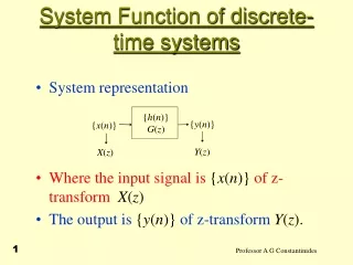
5. 3. Linear time-invariant system • Functional relationship of discrete time system Fig. 6-2. where is impulse response of system

6. The system is said to be linear if • The system is said to be time-invariant if

7. Form and transfer function • Difference equation of discrete time system After z-transform

8. Transfer function If where is impulse response of system

9. Impulse response of discrete time system If is power series In this case,

10. Example 6-3 Using power series

11. Using other method Substitute , and initial value

12. Example 6-4 Using z-transfrom Using inverse z-transfrom

13. If initial value Using inverse z-transfrom

14. System stability • BIBO(bounded input, bounded output)

15. Raible tabulation Table 6-1. Raible’s tabulation

16. If part or all factor is 0 in the first row, then this table is ended • Singular case • Using substitution n th order case

17. Example 6-5

18. Example 6-6

19. Singular case

20. Example 6-7

21. 4. Description of Pole-Zero • Discrete time system transfer function H(z) where K is gain Poles of at : Zeros of at :

22. Description of pole and zero in z-plane Fig. 6-3.

23. Example 6-8 Fig. 6-4.

24. Example 6-9 Fig. 6-5. K=0.2236

25. 5. Frequency response • Frequency response of system • Method for calculation • Method for geometric calculation

26. Example 6-10 • Method for calculation • Substitution of and using Euler’s formular

27. Substitution of

28. Fig. 6-6.

29. Method for geometric calculation Magnitude response Phase response Fig. 6-7.

30. 6. Realization of system Unit delay Adder/subtractor Constant multiplier Branching Signal multiplier Fig. 6-8.

31. Direct form • Direct form 1

32. (a) (b) Fig. 6-9.

33. Direct form 2 Inverse transform poles zeros

34. (a) (b) Fig. 6-10.

35. Example 6-11 • Direct form 1 • Direct form 2

36. (a) (b) Fig. 6-11.

37. Quantization effect of parameters • Quantization error of parameters • Input signal quantization • Accumulation of arithmetic roundoff errors • Coefficient of transfer function quantization

38. Cascade and parallel canonic form • Cascade canonic form or series form first order second order

39. Fig. 6-12. (a) (b) Fig. 6-13.

40. Parallel canonic form first order second order

41. Fig. 6-14.

42. (a) (b) Fig. 6-15.

43. Example 6-12 • Cascade canonic form Quantization error of parameter is decreased

44. Parallel canonic form

45. (a) (b) Fig. 6-16.

46. Example 6-13 Fig. 6-17.

47. Example 6-14 Substitute

48. Fig. 6-18.

49. FIR system • Direct form • Tapped delay line structure or transversal filter Fig. 6-19.

50. Cascade canonic form where Fig. 6-20.