Download
1 / 10
100 likes | 551 Vues
Survival analysis. Aim: modeling and analysis of time-to-event' dataEvents may include all kinds of positive' or negative' eventsSingle and combined endpointsThis presentation includes a first introduction to survival analysis techniques. Events versus censored data. . At the end of the fol

E N D
1. The analysis of survival data: the Kaplan Meier method Kitty J. Jager�, Paul van Dijk1,2, Carmine Zoccali3 and
Friedo W. Dekker1,4
1 ERA�EDTA Registry, Dept. of Medical Informatics, Academic Medical Center, Amsterdam, The Netherlands
2 Department of Clinical Epidemiology, Biostatistics and Bio-informatics, Academic Medical Center,
University of Amsterdam, Amsterdam, The Netherlands
3 CNR�IBIM Clinical Epidemiology and Pathophysiology of Renal Diseases and Hypertension, Renal and Transplantation Unit, Ospedali Riuniti, 89125 Reggio Cal., Italy
4 Department of Clinical Epidemiology, Leiden University Medical Centre, Leiden, The Netherlands
Kidney International: ABC on epidemiology
2. The primary aim of survival analysis is the modeling and analysis of �time-to-event� data; that is data that have as an endpoint the time when an event occurs.
In this respect events are not limited to death, but may include all kinds of �positive� or �negative� events like myocardial infarction, recovery of renal function, first renal transplant, graft failure or time to discharge from hospital.
In addition to these �single� endpoints, an increasing number of studies examine the incidence of a combined or composite endpoint, which can merge a variety of outcomes in one group. For example, the 4-D study used �death from cardiac causes, nonfatal myocardial infarction, and stroke� as their primary outcome, whereas the CREATE trial chose to study the incidence of a �composite of eight cardiovascular events�. Using combined endpoints one addresses event-free survival, an important criterion in therapy evaluation.
This presentation includes a first introduction to survival analysis techniques
The primary aim of survival analysis is the modeling and analysis of �time-to-event� data; that is data that have as an endpoint the time when an event occurs.
In this respect events are not limited to death, but may include all kinds of �positive� or �negative� events like myocardial infarction, recovery of renal function, first renal transplant, graft failure or time to discharge from hospital.
In addition to these �single� endpoints, an increasing number of studies examine the incidence of a combined or composite endpoint, which can merge a variety of outcomes in one group. For example, the 4-D study used �death from cardiac causes, nonfatal myocardial infarction, and stroke� as their primary outcome, whereas the CREATE trial chose to study the incidence of a �composite of eight cardiovascular events�. Using combined endpoints one addresses event-free survival, an important criterion in therapy evaluation.
This presentation includes a first introduction to survival analysis techniques
3. The distinguishing feature of survival data is that at the end of the follow-up period the event will probably not have occurred for all patients. For these patients survival time is said to be censored.
We do not know when or whether such a patient will experience the event of interest, only that he or she has not done so by the end of the observation period.
Censoring may also occur for other reasons. A patient may be lost to follow up during the study or may experience a �competing� event as a result of which further follow-up is impossible. For example, patients being followed for myocardial infarction on dialysis may die of a malignancy. Other cases of censoring are included in the following example on the survival of RRT patients.
Example 1 Survival time on RRT: events and censored observations
Incident RRT patients in the ERA-EDTA Registry were included in an analysis of patient survival on RRT. Like in most survival studies patients were recruited over a period of time (1996-2000 - the inclusion period) and they were observed up to a specific date (31 December 2005 - the end of the follow-up period). During this period the event of interest was �death while on RRT�, whereas censoring took place at recovery of renal function, loss to follow-up and at 31 December 2005. The distinguishing feature of survival data is that at the end of the follow-up period the event will probably not have occurred for all patients. For these patients survival time is said to be censored.
We do not know when or whether such a patient will experience the event of interest, only that he or she has not done so by the end of the observation period.
Censoring may also occur for other reasons. A patient may be lost to follow up during the study or may experience a �competing� event as a result of which further follow-up is impossible. For example, patients being followed for myocardial infarction on dialysis may die of a malignancy. Other cases of censoring are included in the following example on the survival of RRT patients.
Example 1 Survival time on RRT: events and censored observations
Incident RRT patients in the ERA-EDTA Registry were included in an analysis of patient survival on RRT. Like in most survival studies patients were recruited over a period of time (1996-2000 - the inclusion period) and they were observed up to a specific date (31 December 2005 - the end of the follow-up period). During this period the event of interest was �death while on RRT�, whereas censoring took place at recovery of renal function, loss to follow-up and at 31 December 2005.
4. This Figure shows the times that 8 of the patients from this cohort were at risk of death on RRT. Over the period there were 5 events and 3 censored observations. Here one can see the analogy with the concept of incidence rate: these investigators studied the incidence rate (hazard) of death, �the speed of dying�, as the number of deaths was related to the time at risk of death on RRT. This Figure shows the times that 8 of the patients from this cohort were at risk of death on RRT. Over the period there were 5 events and 3 censored observations. Here one can see the analogy with the concept of incidence rate: these investigators studied the incidence rate (hazard) of death, �the speed of dying�, as the number of deaths was related to the time at risk of death on RRT.
5. There are some assumptions related to the use of censoring. The two most important ones will be discussed here.
First, it is assumed that at any time patients who are censored have the same survival prospects as those who continue to be followed. This assumption cannot easily be tested. In the survival of dialysis patients for example it is customary to censor the survival time of a patient at the time of transplantation, because at that time the patient is no longer at risk of death on dialysis. However, we all know that dialysis patients who are placed on the waiting list for transplantation are healthier than those who are not. Therefore, using censoring for transplantation while studying the survival on dialysis is needed, because of the change in treatment, but it in this case probably this first assumption for the use of censoring is not fully fulfilled.
Secondly, survival probabilities are assumed to be the same for subjects recruited early and late in the study. This assumption may be tested, for example by splitting a cohort of patients in those who were recruited early and those recruited late and see if their survival curves are different. There are some assumptions related to the use of censoring. The two most important ones will be discussed here.
First, it is assumed that at any time patients who are censored have the same survival prospects as those who continue to be followed. This assumption cannot easily be tested. In the survival of dialysis patients for example it is customary to censor the survival time of a patient at the time of transplantation, because at that time the patient is no longer at risk of death on dialysis. However, we all know that dialysis patients who are placed on the waiting list for transplantation are healthier than those who are not. Therefore, using censoring for transplantation while studying the survival on dialysis is needed, because of the change in treatment, but it in this case probably this first assumption for the use of censoring is not fully fulfilled.
Secondly, survival probabilities are assumed to be the same for subjects recruited early and late in the study. This assumption may be tested, for example by splitting a cohort of patients in those who were recruited early and those recruited late and see if their survival curves are different.
6. Using survival data investigators often wish to estimate the probability of a patient surviving for a given period like one or two years. In addition, they are also interested to compare the survival of different groups.
The following will elaborate on the method that is most frequently used to calculate survival probabilities, the Kaplan-Meier method.
Example 2 Survival probability in RRT patients due to diabetes mellitus and other causes
In a sample of 50 RRT patients taken from a study on diabetes mellitus survival time started running at the moment a patient was included in the study, in this case at the start of RRT. Patients were followed until death or censoring. The survival probability was calculated using the Kaplan Meier method. Subsequently, the survival of patients with ESRD due to diabetes mellitus was compared to the survival of those with ESRD due to other causes.
Before analysis the observed survival times were first sorted in ascending order, starting with the patient with the shortest survival time.
Using survival data investigators often wish to estimate the probability of a patient surviving for a given period like one or two years. In addition, they are also interested to compare the survival of different groups.
The following will elaborate on the method that is most frequently used to calculate survival probabilities, the Kaplan-Meier method.
Example 2 Survival probability in RRT patients due to diabetes mellitus and other causes
In a sample of 50 RRT patients taken from a study on diabetes mellitus survival time started running at the moment a patient was included in the study, in this case at the start of RRT. Patients were followed until death or censoring. The survival probability was calculated using the Kaplan Meier method. Subsequently, the survival of patients with ESRD due to diabetes mellitus was compared to the survival of those with ESRD due to other causes.
Before analysis the observed survival times were first sorted in ascending order, starting with the patient with the shortest survival time.
7. This resulted in this Table showing the patient deaths and the censored observations over the first 57 days.
By considering time in many small intervals it becomes possible to calculate the probability of surviving a given day. At the start of the study all 50 patients were alive, so the proportion surviving and the cumulative survival (synonym: cumulative proportion surviving) both were 1.00.
When the first patient died on day 34 after the start of RRT, the proportion surviving on that day was 49/50 = 0.9800 = 98%. To calculate the cumulative survival this proportion surviving of 0.9800 was multiplied by the 1.0 cumulative survival from the previous step resulting in a cumulative survival dropping that day to 0.9800.
Then, when the second patient died at day 35, the proportion surviving on that day was 48/49 = 0.9796. To obtain the cumulative survival at day 35, again, this proportion was multiplied by the 0.9800 cumulative survival from the previous step which resulted in a cumulative survival dropping that day to 0.9600. Along the same lines cumulative survival on day 44 dropped to 0.9400.
On day 57, however, a patient was withdrawn alive from the study, because his follow-up time was censored at the end of the study period. The proportion surviving that day was 47/47 = 1.00, as this patient did not die but was withdrawn alive from the study. As a result the cumulative survival did not drop that day but remained unchanged at 0.9400. This resulted in this Table showing the patient deaths and the censored observations over the first 57 days.
By considering time in many small intervals it becomes possible to calculate the probability of surviving a given day. At the start of the study all 50 patients were alive, so the proportion surviving and the cumulative survival (synonym: cumulative proportion surviving) both were 1.00.
When the first patient died on day 34 after the start of RRT, the proportion surviving on that day was 49/50 = 0.9800 = 98%. To calculate the cumulative survival this proportion surviving of 0.9800 was multiplied by the 1.0 cumulative survival from the previous step resulting in a cumulative survival dropping that day to 0.9800.
Then, when the second patient died at day 35, the proportion surviving on that day was 48/49 = 0.9796. To obtain the cumulative survival at day 35, again, this proportion was multiplied by the 0.9800 cumulative survival from the previous step which resulted in a cumulative survival dropping that day to 0.9600. Along the same lines cumulative survival on day 44 dropped to 0.9400.
On day 57, however, a patient was withdrawn alive from the study, because his follow-up time was censored at the end of the study period. The proportion surviving that day was 47/47 = 1.00, as this patient did not die but was withdrawn alive from the study. As a result the cumulative survival did not drop that day but remained unchanged at 0.9400.
8. This example shows that cumulative survival is a probability of surviving the next period multiplied by the probability of having survived the previous period.
Secondly, the example shows that all subjects at risk (also those not experiencing the event during the observation period) can contribute survival time to the denominator of the incidence rate.
Finally, it demonstrates that by censoring one is able to reduce the number of persons alive without affecting the cumulative survival.
The same data were used to construct the survival curve of these 50 patients. The Figure displays visually that cumulative survival drops with every death, whereas it remains unchanged with every censored observation (indicated by the plus signs).This example shows that cumulative survival is a probability of surviving the next period multiplied by the probability of having survived the previous period.
Secondly, the example shows that all subjects at risk (also those not experiencing the event during the observation period) can contribute survival time to the denominator of the incidence rate.
Finally, it demonstrates that by censoring one is able to reduce the number of persons alive without affecting the cumulative survival.
The same data were used to construct the survival curve of these 50 patients. The Figure displays visually that cumulative survival drops with every death, whereas it remains unchanged with every censored observation (indicated by the plus signs).
9. When we go back to the previous table we can see the median survival.
The median survival is that point in time, from the time of inclusion, when the cumulative survival drops below 50%, in this case it is 1708 days. Please, note the median survival is not related to the number of deaths or to the number of subjects that is still at risk of death.
In general, investigators use median survival rather than mean survival. There are a number of reasons for this:
The first one is that samples of survival times are mostly highly skewed and in those cases the median is generally a better measure of central location than the mean.
A second reason is that in survival analysis one makes use of censoring. As we explained earlier one does not know when or whether such a person will experience the event of interest, only that he or she has not done so by the end of the observation period. This complicates the calculation of the mean.
Finally, even in cases where there is no censoring, in order to calculate a mean one would need to wait until all persons reached the event of interest and this may require quite a long period.
For these reasons it is simpler to use median survival, as this is completely defined once the survival curve descends to 50%.
When we go back to the previous table we can see the median survival.
The median survival is that point in time, from the time of inclusion, when the cumulative survival drops below 50%, in this case it is 1708 days. Please, note the median survival is not related to the number of deaths or to the number of subjects that is still at risk of death.
In general, investigators use median survival rather than mean survival. There are a number of reasons for this:
The first one is that samples of survival times are mostly highly skewed and in those cases the median is generally a better measure of central location than the mean.
A second reason is that in survival analysis one makes use of censoring. As we explained earlier one does not know when or whether such a person will experience the event of interest, only that he or she has not done so by the end of the observation period. This complicates the calculation of the mean.
Finally, even in cases where there is no censoring, in order to calculate a mean one would need to wait until all persons reached the event of interest and this may require quite a long period.
For these reasons it is simpler to use median survival, as this is completely defined once the survival curve descends to 50%.
10. The logrank test is the most popular method of comparing the survival of groups.
It takes the whole follow-up period into account and it addresses the hypothesis that there are no differences between the populations being studied in the probability of an event at any time point.
The test is based on the same assumptions as the Kaplan Meier method.�The logrank test is the most popular method of comparing the survival of groups.
It takes the whole follow-up period into account and it addresses the hypothesis that there are no differences between the populations being studied in the probability of an event at any time point.
The test is based on the same assumptions as the Kaplan Meier method.�
11. The Kaplan Meier method is the most popular method used for survival analysis. Together with the logrank test it may provide us with an opportunity to estimate survival probabilities and to compare survival between groups.
Most of the time, however, one would like to do more than that: one would like to be informed on the size of any potential difference and to adjust for age and other confounding variables.
However, as the logrank test is purely a significance test, it cannot provide an estimate of the size of the difference between groups and a related confidence interval.
Secondly, the Kaplan Meier method and the logrank test can only study the effect of one factor at the time and therefore they cannot be used for multivariate analysis.
For these purposes one may use a regression technique like the Cox proportional hazards model, which will be described in the next paper in this series. The Kaplan Meier method is the most popular method used for survival analysis. Together with the logrank test it may provide us with an opportunity to estimate survival probabilities and to compare survival between groups.
Most of the time, however, one would like to do more than that: one would like to be informed on the size of any potential difference and to adjust for age and other confounding variables.
However, as the logrank test is purely a significance test, it cannot provide an estimate of the size of the difference between groups and a related confidence interval.
Secondly, the Kaplan Meier method and the logrank test can only study the effect of one factor at the time and therefore they cannot be used for multivariate analysis.
For these purposes one may use a regression technique like the Cox proportional hazards model, which will be described in the next paper in this series.