Download
1 / 50
500 likes | 739 Vues
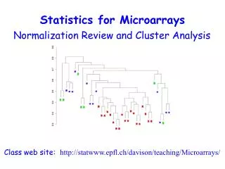
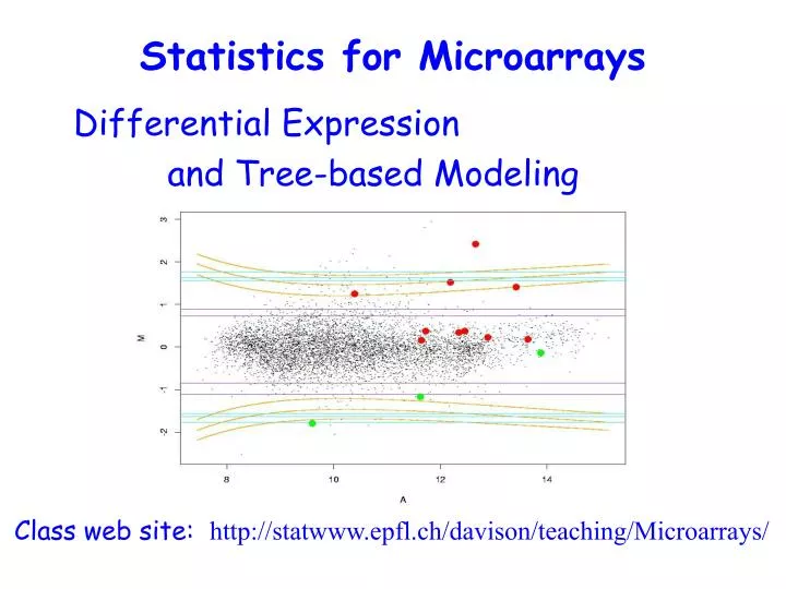
Statistics for Microarrays. Differential Expression and Tree-based Modeling. Class web site: http://statwww.epfl.ch/davison/teaching/Microarrays/. cDNA gene expression data. mRNA samples. Data on G genes for n samples. sample1 sample2 sample3 sample4 sample5 …

E N D
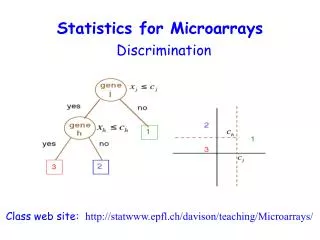
Statistics for Microarrays Differential Expression and Tree-based Modeling Class web site: http://statwww.epfl.ch/davison/teaching/Microarrays/
cDNA gene expression data mRNA samples Data on G genes for n samples sample1 sample2 sample3 sample4 sample5 … 1 0.46 0.30 0.80 1.51 0.90 ... 2 -0.10 0.49 0.24 0.06 0.46 ... 3 0.15 0.74 0.04 0.10 0.20 ... 4 -0.45 -1.03 -0.79 -0.56 -0.32 ... 5 -0.06 1.06 1.35 1.09 -1.09 ... Genes Gene expression level of gene i in mRNA samplej = (normalized) Log(Red intensity / Green intensity)
Identifying Differentially Expressed Genes • Goal: Identify genes associated with covariate or response of interest • Examples: • Qualitative covariates or factors: treatment, cell type, tumor class • Quantitative covariate: dose, time • Responses: survival, cholesterol level • Any combination of these!
Differentially Expressed Genes • Simultaneously test m null hypotheses, one for each gene j : Hj: no association between expression level of gene j and covariate/response • Combine expression data from different slides and estimate effects of interest • Compute test statistic Tj for each gene j • Adjust for multiple hypothesis testing
Test statistics • Qualitative covariates: e.g. two-sample t-statistic, Mann-Whitney statistic, F-statistic • Quantitative covariates: e.g. standardized regression coefficient • Survival response: e.g. score statistic for Cox model
QQ-Plot Sample Used to assess whether a sample follows a particular (e.g. normal) distribution (or to compare two samples) A method for looking for outliers when data are mostly normal Recall that for the normal distribution, approximately: 68% within 1 SD of the mean 95% within 2 SDs 99.7% within 3 SDs Sample quantile is 0.125 Theoretical Value from Normal distribution which yields a quantile of 0.125 (= -1.15)
Typical Deviations from Straight Line Patterns • Outliers • Curvature at both ends (long or short tails) • Convex/concave curvature (asymmetry) • Horizontal segments, plateaus, gaps
Example: Apo AI experiment(Callow et al., Genome Research, 2000) GOAL: Identify genes with altered expression in the livers of one line of mice with very low HDL cholesterol levels compared to inbred control mice Experiment: • Apo AI knock-out mouse model • 8 knockout (ko) mice and 8 control (ctl) mice (C57Bl/6) • 16 hybridisations: mRNA from each of the 16 mice is labelled with Cy5, pooled mRNA from control mice is labelled with Cy3 Probes: ~6,000 cDNAs, including 200 related to lipid metabolism
Which genes have changed? This method can be used with replicated data: 1. For each gene and each hybridisation (8 ko + 8 ctl) use M=log2(R/G) 2. For each gene form the t-statistic: average of 8 ko Ms - average of 8 ctl Ms sqrt(1/8 (SD of 8 ko Ms)2 + 1/8 (SD of 8 ctl Ms)2) 3. Form a histogram of 6,000 t values 4. Make a normal Q-Q plot; look for values “off the line” 5. Adjust for multiple testing
Histogram & Q-Q plot ApoA1
Assigning p-values to measures of change • Estimate p-values for each comparison (gene) by using the permutation distribution of the t-statistics. • For each of the possible permutation of the trt / ctl labels, compute the two-sample t-statistics t* for each gene. • The unadjusted p-value for a particular gene is estimated by the proportion of t*’s greater than the observed t in absolute value.
Multiple Testing * Per-comparison = E(V)/m * Family-wise = p(V ≥ 1) * Per-family = E(V) * False discovery rate = E(V/R)
Apo AI: Adjusted and unadjusted p-values for the 50 genes with the larges absolute t-statistics
Single-slide methods • Model-dependent rules for deciding whether (R,G) corresponds to a differentially expressed gene • Amounts to drawing two curves in the (R,G)-plane; call a gene differentially expressed if it falls outside the region between the two curves • At this time, not enough known about the systematic and random variation within a microarray experiment to justify these strong modeling assumptions • n = 1 slide may not be enough (!)
Single-slide methods • Chen et al: Each (R,G) is assumed to be normally and independently distributed with constant CV; decision based on R/G only (purple) • Newton et al: Gamma-Gamma-Bernoulli hierarchical model for each (R,G) (yellow) • Roberts et al: Each (R,G) is assumed to be normally and independently distributed with variance depending linearly on the mean • Sapir & Churchill: Each log R/G assumed to be distributed according to a mixture of normal and uniform distributions; decision based on R/G only (turquoise)
Difficulty in assigning valid p-values based on a single slide Matt Callow’s Srb1 dataset (#8). Newton’s, Sapir & Churchill’s and Chen’s single slide method
Another example: Survival analysis with expression data • Bittner et al. looked at differences in survival between the two groups (the ‘cluster’ and the ‘unclustered’ samples) • ‘Cluster’ seemed to have longer survival
Average Linkage Hierarchical Clustering, survival only unclustered cluster
Identification of genes associated with survival For each gene j, j = 1, …, 3613, model the instantaneous failure rate, or hazard function, h(t) with the Cox proportional hazards model: h(t) = h0(t)exp(jxij) • and look for genes with both: • large effect size j • large standardized effect size j/SE(j) ^ ^ ^
Findings • Top 5 genes by this method not in Bittner et al. ‘weighted gene list’ - Why? • weighted gene list based on entire sample; our method only used half • weighting relies on Bittner et al. cluster assignment • other possibilities?
Limitations of Single Gene Tests • May be too noisy in general to show much • Do not reveal coordinated effects of positively correlated genes • Hard to relate to pathways
Some ideas for further work • Expand models to include more genes and possibly two-way interactions • Nonparametric tree-based subset selection – would require much larger sample sizes
Trees • Provide means to express knowledge • Can aid in decision making • Can be portrayed graphically or by means of a chart or ‘key’, e.g. (MASS space shuttle):
Tree-based Methods – References • Hastie, Tibshirani, Friedman 2001 • The Elements of Statistical Learning • Venables and Ripley, 1999 • Modern Applied Statistics with S-Plus (MASS) • Ripley, 1996 • Pattern Recognition and Neural Networks • Breiman, Olshen, Friedman, Stone 1984 • Classification and Regression Trees
Tree-based Methods • Automatic construction of decision trees dates from social science work in the early 1960’s (AID) • Breiman et al. (1984) proposed new algorithms for tree construction (CART) • Tree construction can be seen as a type of variable selection
Response types • Categorical outcome – Classification tree • Continuous outcome – Regression tree • Survival outcome – Survival tree • Software – Available R packages include tree, rpart (tssa available in S)
Trees Partition the Feature Space • End point of tree is a (labeled) partition of the (feature) space of possible observations X • Tree-based methods partition X into rectangular regions; try to make the (average) responses in each box as different as possible • In logical problems it is assumed that there does exist a partition of X that will correctly classify all observations; task is to find a tree to succinctly describe this partition
Partitions and CART Yes No XX R5 R2 t4 X2 X2 XX R3 t2 XX R4 R1 t1 t3 X1 X1
Partitions and CART X1 t1 R5 R2 X2 t2 X1 t3 t4 X2 R3 t2 X2 t4 R4 R1 R1 R2 R3 t1 t3 R4 R5 X1
Tree Comparison • Measure how well the partition created by a tree corresponds to the correct decision rule (classification) • For a logical problem, count number errors • For statistical problem, usually overlapping class distributions, so that no partition unambiguously describes classes – estimate misclassification prob.
Three Aspects of Tree Construction • Split Selection Rule • Split-stopping Rule • Assignment of predicted values
Split Selection • Binary splits • Look only one step ahead – avoids massive computational time by not attempting to optimize whole tree performance • Choose an impurity measure to optimize each split – Gini index or entropy, rather than misclassification rate for classification tree, deviance (squared error) for regression tree
Split-stopping • Issue: A very large tree will tend to overfit the data (and therefore lack generalizability), while too small a tree might not capture important structure • Usual solution: grow large/maximal tree (stop splitting only when some minimum node size, 5 or 10 say, is reached), followed by (cost-complexity) pruning
Pruning • Sequence of rooted subtrees • Measure Ri (e.g. deviance) at leaves, R = Ri • Minimize the cost-complexity measure R = R + * size • governs tradeoff between tree size and goodness of fit • Choose to minimize cross-validated error (misclassification or deviance)
Assignment of Predicted Values • Assign value to each leaf (terminal node) • In Classification: (weighted) voting among observations in the node • In Regression: mean of observations in the node
Other Issues (I) • Loss matrix – Procedures can be modified for asymmetric losses • Missing predictor values • Can create ‘missing’ category • Surrogate splits exploit correlation between predictors • Linear combination splits
Other Issues (II) • Tree Instability • Small changes in the data can result in very different series of splits – difficulties in interpretation • Aggregate trees to reduce (e.g. bagging) • Lack of smoothness • More of an issue in regression trees • Multivariate Adaptive Regression Splines (MARS) • Difficulty in capturing additive structure with binary trees
Acknowledgements • Sandrine Dudoit • Jane Fridlyand • Yee Hwa (Jean) Yang • Debashis Ghosh • Erin Conlon • Ingrid Lonnstedt • Terry Speed