Download
1 / 53
550 likes | 888 Vues
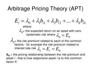
Department of Banking and Finance. SPRING 200 7 -0 8. Capital Asset Pricing and Arbitrage Pricing Theory. by Asst. Prof. Sami Fethi. Capital Asset Pricing Model (CAPM).

E N D
Department of Banking and Finance SPRING 2007-08 Capital Asset Pricing and Arbitrage Pricing Theory by Asst. Prof. Sami Fethi
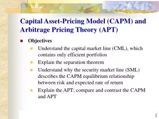
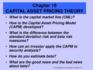
Capital Asset Pricing Model (CAPM) • The asset pricing models aim to use the concepts of portfolio valuation and market equilibrium in order to determine the market price for risk and appropriate measure of risk for a single asset. • Capital Asset Pricing Model (CAPM) has an observation that the returns on a financial asset increase with the risk. CAPM concerns two types of risk namely unsystematic and systematic risks. The central principle of the CAPM is that, systematic risk, as measured by beta, is the only factor affecting the level of return.
Capital Asset Pricing Model (CAPM) • The Capital Asset Pricing Model (CAPM) was developed independently by Sharpe (1964), Lintner (1965) and Mossin (1966) as a financial model of the relation of risk to expected return for the practical world of finance. • CAPM is originally depending on the mean variance theory which was demonstrated by Markowitz’s portfolio selection model (1952) aiming higher average returns with lower risk.
Capital Asset Pricing Model (CAPM) • Equilibrium model that underlies all modern financial theory • Derived using principles of diversification with simplified assumptions • Markowitz, Sharpe, Lintner and Mossin are researchers credited with its development
Capital Asset Pricing Model (CAPM) • From the point that most of the investors think that the variance or standard deviation of their portfolio’s return will enable them to quantify the risk, portfolio selection model is used in order to find the efficient portfolios and secondly to generate an equation that relates the risk of an asset to its expected return. • The reason for this is that portfolios are expected to have maximum return given the variance of future returns. Therefore, Mean Variance Analysis is one of the tools for achieving higher average returns with lower risk and as a second tool Capital Asset Pricing Model’s main parameters are depending on mean and variance of returns.
Capital Asset Pricing Model (CAPM) • Moreover, CAPM requires that in the equilibrium the market portfolio must be an efficient portfolio. One way to establish its efficiency is to argue that if investors have homogenous expectations, the set of optimal portfolios they would face would be using the same values of expected returns, variances and co variances. • Therefore, the efficiency of the market portfolio and the CAPM are joint hypothesis and it is not possible to test the validity of one without the other (Roll, 1977).
CAPM Assumptions-Summary • Individual investors are price takers • Single-period investment horizon • Investments are limited to traded financial assets • No taxes, and transaction costs • Information is costless and available to all investors • Investors are rational mean-variance optimizers • Homogeneous expectations
Assumptions • Asset markets are frictionless and information liquidity is high. • All investors are price takers; so that, they are not able to influence the market price by their actions. • All investors have homogenous expectations about asset returns and what the uncertain future holds for them. • All investors are risk averse and they operate in the market rationally and perceive utility in terms of expected return.
Assumptions (cont.) • All investors are operating in perfect markets which enables them to operate without tax payments on returns and without cost of transactions entailed in trading securities. • All securities are highly divisible for instance they can be traded in small parcels (Elton and Gruber, 1995, p.294). • All investors can lend and borrow unlimited amount of funds at the risk-free rate of return. • All investors have single period investment time horizon in means of different expectations from their investments leads them to operate for short or long term returns from their investments.
Resulting Equilibrium Conditions • All investors will hold the same portfolio for risky assets – market portfolio • Market portfolio contains all securities and the proportion of each security is its market value as a percentage of total market value • Risk premium on the market depends on the average risk aversion of all market participants • Risk premium on an individual security is a function of its covariance with the market
Capital Market Line E(r) CML M E(rM) rf s sm
Capital Market Line • If a fully diversified investor is able to invest in the market portfolio and lend or borrow at the risk free rate of return, the alternative risk and return relationships can be generally placed around a market line which is called the Capital Market Line (CML).
Capital Market Line • CML: E(rp)= rF+ λσp • E(rp): Expected return on portfolio • rF : Return on the risk free asset • λ : Market price risk • σp : Market portfolio risk
Slope and Market Risk Premium M = Market portfolio rf = Risk free rate E(rM) - rf = Market risk premium E(rM) - rf = Market price of risk = Slope of the CAPM s M
Expected Return and Risk on Individual Securities • The risk premium on individual securities is a function of the individual security’s contribution to the risk of the market portfolio • Individual security’s risk premium is a function of the covariance of returns with the assets that make up the market portfolio
Security Market Line • The SML shows the relationship between risk measured by beta and expected return. The model states that the stock’s expected return is equal to the risk-free rate plus a risk premium obtained by the price of the risk multiplied by the quantity of the risk.
Security Market Line E(r) SML E(rM) rf ß ß = 1.0 M
SML Relationships b = [COV(ri,rm)] / sm2 Slope SML = E(rm) - rf = market risk premium SML = rf + b[E(rm) - rf] SML: E(rS)=rF+ λσSpS,M (σSpS,M)is the market price of risk
Sample Calculations for SML E(rm) - rf = .08 rf = .03 bx = 1.25 E(rx) = .03 + 1.25(.08) = .13 or 13% by = .6 e(ry) = .03 + .6(.08) = .078 or 7.8%
Graph of Sample Calculations E(r) SML Rx=13% .08 Rm=11% Ry=7.8% 3% ß .6 1.0 1.25 ß ß ß y m x
Disequilibrium Example • Suppose a security with a beta of 1.25 is offering expected return of 15% • According to SML, it should be 13% • Underpriced: offering too high of a rate of return for its level of risk
Disequilibrium Example E(r) SML 15% Rm=11% rf=3% ß 1.0 1.25
Security Characteristic Line Excess Returns (i) SCL . . . . . . . . . . . . . . . . . . . . . . . . . . Excess returns on market index . . . . . . . . . . . . . . . . . . . . . . . . Ri = ai + ßiRm + ei
Using the Text Example p. 231, Table 7.5 Excess GM Ret. Excess Mkt. Ret. Jan. Feb. . . Dec Mean Std Dev 5.41 -3.44 . . 2.43 -.60 4.97 7.24 .93 . . 3.90 1.75 3.32
Regression Results: a rGM - rf = + ß(rm - rf) a ß Estimated coefficient Std error of estimate Variance of residuals = 12.601 Std dev of residuals = 3.550 R-SQR = 0.575 -2.590 (1.547) 1.1357 (0.309)
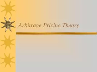
Arbitrage Pricing Theory • Arbitrage Pricing Theory was developed by Stephen Ross (1976). His theory begins with an analysis of how investors construct efficient portfolios and offers a new approach for explaining the asset prices and states that the return on any risky asset is a linear combination of various macroeconomic factors that are not explained by this theory namely. • Similar to CAPM it assumes that investors are fully diversified and the systematic risk is an influencing factor in the long run. However, unlike CAPM model APT specifies a simple linear relationship between asset returns and the associated factors because each share or portfolio may have a different set of risk factors and a different degree of sensitivity to each of them.
The Assumptions of APT • Capital asset returns’ properties are consistent with a linear structure of the factors. The returns can be described by a factor model. • Either there are no arbitrage opportunities in the capital markets or the markets have perfect competition. • The number of the economic securities are either inestimable or so large that the law of large number can be applied that makes it possible to form portfolios that diversify the firm specific risk of individual stocks. • Lastly, the number of the factors can be estimated by the investor or known in advance (K. C. John Wei, 1988)
The Model of APT k • Ri= E( Ri )+ ∑ δj βij+εi j=1 • where, • R i : The single period expected rate on security i , i =1,2….,n • δj : The zero mean j factor common to the all assets under consideration • βij : The sensitivity of security i’s returns to the fluctuations in the j th common factor portfolio • εi : A random of i th security that constructed to have a mean of zero.
Arbitrage Pricing Theory-briefly • Arbitrage - arises if an investor can construct a zero investment portfolio with a sure profit • Since no investment is required, an investor can create large positions to secure large levels of profit • In efficient markets, profitable arbitrage opportunities will quickly disappear
Arbitrage Example Current Expected Standard Stock Price$ Return% Dev.% A 10 25.0 29.58 B 10 20.0 33.91 C 10 32.5 48.15 D 10 22.5 8.58
Arbitrage Portfolio Mean Stan. Correlation Return Dev. Of Returns Portfolio A,B,C 25.83 6.40 0.94 D 22.25 8.58
Arbitrage Action and Returns E. Ret. * P * D St.Dev. Short 3 shares of D and buy 1 of A, B & C to form P You earn a higher rate on the investment than you pay on the short sale
APT and CAPM Compared • APT applies to well diversified portfolios and not necessarily to individual stocks • With APT it is possible for some individual stocks to be mispriced - not lie on the SML • APT is more general in that it gets to an expected return and beta relationship without the assumption of the market portfolio • APT can be extended to multifactor models
Example-market risk • Suppose the risk free rate is 5%, the average investor has a risk-aversion coefficient of A* is 2, and the st. dev. Of the market portfolio is 20%. • A) Calculate the market risk premium. • B) Find the expected rate of return on the market. • C) Calculate the market risk premium as the risk-aversion coefficient of A* increases from 2 to 3. • D) Find the expected rate of return on the market referring to part c.
Answer-market risk • A) E(rm-rf)=A*σ2m • Market Risk Premium =2(0.20)2=0.08 • B) E(rm) = rf +Eq. Risk prem • =0.05+0.08=0.13 or 13% • C) Market Risk Premium =3(0.20)2=0.12 • D) E(rm) = rf +Eq. Risk prem • =0.05+0.12=0.17 or 17%
Example-risk premium • Suppose an av. Excess return over Treasury bill of 8% with a st. dev. Of 20%. • A) Calculate coefficient of risk-aversion of the av. investor. • B) Calculate the market risk premium as the risk-aversion coefficient is 3.5
Answer-risk premium • A) A*= E(rm-rf)/ σ2m =0.085/0.202=2.1 • B) E(rm)-rf =A*σ2m =3.5(0.20)2=0.14 or 14%
Example-EROR • Suppose the risk premium of the market portfolio is 9%, and the estimated beta is 1.3. The risk premium for stock is 1.3 times the market risk premium. • A) Calculate expected ROR if T-bill rate is 5%. • B) Calculate ROR and the risk premium if the estimated of the beta is 1.2 for the company. • C) Find the company’s risk premium if market risk premium and beta are 8% and 1.3 respectively.
Answer-EROR • A) E(rc)=rf+βc[E(rm-rf)] • =5%+1.3(9%)=16.7% • B) E(rc)=rf+βc[E(rm-rf)] • =5%+1.2(9%)=15.8% • 1.2(9%)=10.8% risk premium • C) 1.3(8%)=10.4%
Asset Beta Risk prem. Portfolio Weight X 1.2 9% 0.5 Y 0.8 6 0.3 Z 0.0 0 0.2 Port. 0.84 1.0 Example-Portfolio beta and risk premium • Consider the following portfolio: • A) Calculate the risk premium on each portfolio • B) Calculate the total portfolio if Market risk premium is 7.5%.
Answer-Portfolio beta and risk premium • A) (9%) (0.5)=4.5 • (6%) (0.3)=1.8 • =6.3% • B) 0.84(7.5)=6.3%
Example-risk premium • Suppose the risk premium of the market portfolio is 8%, with a st. dev. Of 22%. • A) Calculate portfolio’s beta. • B) Calculate the risk premium of the portfolio referring to a portfolio invested 25% in x motor company with beta 0f 1.15 and 75% in y motor company with a beta of 1.25.
Answer-risk premium • A) βy= 1.25, βx= 1.15 • βp=wy βy+ wx βx • =0.75(1.25)+0.25(1.15)=1.225 • B) E(rp)-rf=βp[E(rm)-rf] • =1.225(8%)=9.8%
Example-SML • Suppose the return on the market is expected to be 14%, a stock has a beta of 1.2, and the T-bill rate is 6%. • A) Calculate the expected return of the SML • B) If the return is 17%, calculate alpha of the stock
Answer-SML E(r) Stock SML • A) E(rp)=rf+β[E(rm)-rf] • =6+1.2(14-6)=15.6% 17% 15.6% α= 17-15.6=1.4 14% M 6% ß 1.0 1.2
Example-SML • Stock xyz has an expected return of 12% and risk of beta is 1.5. Stock ABC is expected to return 13% with a beta of 1.5. The market expected return is 11% and rf=5%. • A) Based on CAPM, which stock is a better buy? • B) What is the alpha of each stock? • C) Plot the relevant SML of the two stocks • D) rf is 8% ER on the market portfolio is 16%, and estimated beta is 1.3, what is the required ROR on the project? • E) If the IRR of the project is 19%, what is the project alpha?
Answer-SML • A and B) α=E(r)-{rf+β[E(rm)-rf]} • αXYZ= 12-{5+1.0[11-5]}=1 • UNDERVALUED • αABC= 13-{5+1.5[11-5]}= -1 • OVERVALUED
Answer-SML-C E(r) Stock SML 14% 13% α= 13-14=-1 ABC 12% α =13-12=1 xyz 5% ß 1.0 1.5
Answer-SML • D) E(r)={rf+β[E(rm)-rf]} • = 8+1.3[16-8]=18.4% • E) If the IRR of the project is 19%, it is desirable. However, any project with an IRR by using similar beta is less than 18.4% should be rejected.
Market Return Aggressive stock Defensive stock 5% 2% 3.5% 20 32 14 Example-SML • Consider the following table: