Download
1 / 30
330 likes | 713 Vues
Economics 105: Statistics. Please practice your RAP, so you can keep it to 7 minutes. We have lots of them to do. please copy your Powerpoint file to your stats P:economicsEco 105 (Statistics) Foley userid lab space.

E N D
Economics 105: Statistics Please practice your RAP, so you can keep it to 7 minutes. We have lots of them to do. please copy your Powerpoint file to your stats P:\economics\Eco 105 (Statistics) Foley\userid\ lab space. Tue Apr 24: Thompson, Shanor, Nielsen, Moniz-Soares, Maher, Dugan, Burke, Adabayeri Thur Apr 26: Ryger-Wasserman, Lockwood, Gordon, Givens, Christ, Blasey, Bernert, Avinger Tue May 1: Yearwood, Swany, Ream, Polak, Pettiglio, Murray, Esposito, Bajaj Thur May 3: Yan, Tompkins, Mwangi, Mooney, Lockhart, Clune, Charles, Bourgeois Review #3 due Monday May 7, by 4:30 PM.
Breusch-Pagan test Estimate the model by OLS Obtain the squared residuals, Run 4. Do the whole model F-test, rejection indicates heteroskedasticity. Assumes Breusch, T.S. and A.R. Pagan (1979), “A Simple Test for Heteroskedasticity and Random Coefficient Variation,”Econometrica 50, pp. 987 - 1000.
Breusch-Pagan test (not needing ) Estimate the model by OLS Obtain the squared residuals, Run keeping the R2 from this regression, call it Test statistic Rejection indicates heteroskedasticity. .
White test Estimate the model by OLS Obtain the squared residuals, Estimate 4. Do the whole model F-test, rejection indicates heteroskedasticity White, H. (1980), “A Heteroskedasticity-Consistent Covariance Matrix Estimator and a Direct Test for Heteroskedasticity,”Econometrica 48, pp. 817 - 838.
White test Adds squares & cross products of all X’s Advantages no assumptions about the nature of the het. Disadvantages Rejection (a statistically significant White test statistic) may be caused by het or it may be due to specification error; it’s a nonconclusive test Number of covariates rises quickly so could also run since the predicted values are functions of the X’s (and the estimated parameters) and do F-test
Violations of GM Assumptions Assumption Violation Wrong functional form Omit Relevant Variable (Include Irrelevant Var) Errors in Variables Sample selection bias, Simultaneity bias “well-specified model” (1) & (5) constant, nonzero mean due to systematically +/- measurement error in Y can only assess theoretically zero conditional mean of errors (2) Homoskedastic errors (3) Heteroskedastic errors No serial correlation in errors (4) There exists serial correlation in errors
Time Series: Multiple Regression Assumptions (1) Linear function in the parameters, plus error Variation in Y is caused by , the error (as well as X) (2) Sources of error Idiosyncratic, “white noise” Measurement error on Y Omitted relevant explanatory variables If (2) holds, we have exogenous explanatory vars If some Xj is correlated with error term for some reason, then that Xj is an endogenous explanatory var
Time Series:Multiple Regression Assumptions (3) Homoskedasticity (4) No autocorrelation (5) Errors and the explanatory variables are uncorrelated (6) Errors are i.i.d. normal
Time Series: Multiple Regression Assumption (7) No perfect multicollinearity no explanatory variable is an exact linear function of other X’s Venn diagram Other implicit assumptions data are a random sample of n observations from proper population n > K the little xij’s are fixed numbers (the same in repeated samples) or they are realizations of random variables, Xij, that are independent of error term & then inference is done CONDITIONAL on observed values of xij’s
Violation of (4) • Error in period t is a function of error in prior period alone: first-order autocorrelation, denoted AR(1) for “autoregressive” process • Usual assumptions apply to new error term • is positive serial correlation • is negative serial correlation Nature of Serial Correlation
Error in period t can be a function of error in more than one prior period • Second-order serial correlation • Higher orders generated analogously • Seasonally-based serial correlation Nature of Serial Correlation
The error term in the regression captures • Measurement error • Omitted variables, that are uncorrelated with the included explanatory variables (hopefully) • Frequently factors omitted from the model are correlated over time • Persistence of shocks • Effects of random shocks (e.g., earthquake, war, labor strike) often carry over through more than one time period • Inertia • times series for GNP, (un)employment, output, prices, interest rates, etc. follow cycles, so that successive observations are related Causes of Serial Correlation
3. Lags • Past actions have a strong effect on current ones • Consumption last period predicts consumption this period • 4. Misspecified model, incorrect functional form • 5. Spatial serial correlation • In cross-sectional data on regions, a random shock in one region can cause the outcome of interest to change in adjacent regions • “Keeping up with the Joneses” Causes of Serial Correlation
Consequences for OLS Estimates • Using an OLS estimator when the errors are autocorrelated results in unbiased estimators • However, the standard errors are estimated incorrectly • Whether the standard errors are overstated or understated depends on the nature of the autocorrelation • For positive AR(1), standard errors are too small! • Any hypothesis tests conducted could yield erroneous results • For positive AR(1), may conclude estimated coefficients ARE significantly different from 0 when we shouldn’t ! • OLS is no longer BLUE • A pattern exists in the errors • Suggesting an estimator that exploited this would be more efficient
Graphical Detection of Serial Correlation
Graphical no obvious pattern—the errors seem random. Sometimes, however, the errors follow a pattern—they are correlated across observations, creating a situation in which the observations are not independent with one another. Detection of Serial Correlation
Detection of Serial Correlation Here the residuals do not seem random, but rather seem to follow a pattern.
Detection: The Durbin-Watson Test • Provides a way to test H0: = 0 • It is a test for the presence of first-order serial correlation • The alternative hypothesis can be • 0 • > 0: positive serial correlation • Most likely alternative in economics • < 0: negative serial correlation • DW Test statistic is d
Detection: The Durbin-Watson Test • To test for positive serial correlation with the Durbin-Watson statistic, under the null we expect d to be near 2 • The smaller d, the more likely the alternative hypothesis The sampling distribution of d depends on the values of the explanatory variables. Since every problem has a different set of explanatory variables, Durbin and Watson derived upper and lower limits for the critical value of the test.
Detection: The Durbin-Watson Test • Durbin and Watson derived upper and lower limits such that d1d* du • They developed the following decision rule
Detection: The Durbin-Watson Test • To test for negative serial correlation the decision rule is • Can use a two-tailed test if there is no strong prior belief about whether there is positive or negative serial correlation—the decision rule is
Serial Correlation Table of critical values for Durbin-Watson statistic (table E11, page 833 in BLK textbook) http://hadm.sph.sc.edu/courses/J716/Dw.html
Serial Correlation Example What is the effect of the price of oil on the number of wells drilled in the U.S.?
Serial Correlation Example What is the effect of the price of oil on the number of wells drilled in the U.S.?
Serial Correlation Example Analyze residual plots … but be careful …
Serial Correlation Example Remember what serial correlation is … • This plot only “works” if obs number is in same order as the unit of time
Serial Correlation Example Same graph when plot versus “year” • Graphical evidence of serial correlation
Serial Correlation Example Calculate DW test statistic Compare to critical value at chosen sig level dlower or dupper for 1 X-var & n = 62 not in table dlower for 1 X-var & n = 60 is 1.55, dupper = 1.62 • Since .192 < 1.55, reject H0: = 0 in favor of H1: > 0 at α=5%