Download
1 / 28
280 likes | 408 Vues
Basic Approach to Mapping Different Sources, and the Sources of Spatial Datasets. John van Aardenne jva@eea-europa.eu. Outline. Introduction Reporting requirements 3. Wake up quiz 4. Post-processing of national inventory data 5. Gridding: concepts and datasets

E N D
Basic Approach to Mapping Different Sources, and the Sources of Spatial Datasets John van Aardenne jva@eea-europa.eu
Outline • Introduction • Reporting requirements 3. Wake up quiz 4. Post-processing of national inventory data 5. Gridding: concepts and datasets 6. Gridding: how does it work in practice 7. Visualization
1. Introduction This presentation is aimed at providing a basic overview for those new or relatively new to emission gridding. Disclaimer: Your presenter is not a GIS expert, nor a programmer, but with common sense, database knowledge and nice GIS colleagues managed to work on spatially resolved emission inventories starting from simple scaling emissions with population (Moguntia model Nox emissions), to EDGAR-HYDE AP and GHG emissions (1x1 degree), Historical AP and GHG emissions for IPCC AR5 (0.5 degree) and EDGARv4 (0.1 degree). So there is hope.....
2. Reporting requirements: EMEP grid Number of grid cells: ~21000 • Size of grid cell • at 40°N (Italy): 40x40 km2 • at 60°N (Scandinavia): 50x50 km2 Extendedd 50 x 50 km2 grid
2. Reporting requirements: sectors A. Public power B. Industrial comb. plants C. Small combustion plants D. Industrial process E. Fugitive emissions F. Solvents G. Road – rail H. Shipping • Off road mobile • J. Civil aviation (domestic lto) • K. Civil aviation (domest cruise) L. Other waste displacement M. Wastewater N. Waste incineration O. Agricultural livestock P. Agriculture (other) Q. Agricultural wastes R. Other S. Natural T. International aviation (cruise) z. Memo
wake up quiz Imagine the emep grid........
3a. The following grid cells represent…… • Hungary • Austria • Latvia
3b. The following grid cells represent…… • Malta • Liechtenstein • Luxembourg
3c. The following grid cells represent…… • Belgium • The Netherlands • Turkey
4. Post-processing of emission inventory data: Emission inventories as annual total by sector are not sufficient to allow for atmospheric chemistry modeling The EMEP unified model has 20 height layers (www.emep.int) Seinfeld, J.H. and Pandis, S.N., Atmospheric chemistry and physics: from air pollution to climate change, Wiley and Sons, New York, 969-971, 1998.
4. Post-processing of emission inventory data: 3 activities are needed. Horizontal allocation: assigning emissions to their proper grid cell using gridded data on spatial surrogates with known geographic distributions Vertical allocation: assigning emissions to their proper layer in the atmosphere. Often static vertical distribution factors are applied to the emissions of each sector or all emissions are put into the lowest layer. Temporal allocation: representing emissions variation over time (closure of facilities for maintenance, rush hour, weekends, public holidays) Source: US EPA emissions modeling clearinghouse, Bieser et al., 2011.
5. Gridding: conceptual Point source: an emission source at a known location such as an industrial plant or a power station. (could be an LPS, or not, depending on threshold) Area source: sources that are too numerous or small to be individually identified as point sources or from which emissions arise over a large area (agricultural fields, residential areas, forests) The grid cells representing the geographic domain for which you have emissions data. Line source: source that exhibits a line type of geography, e.g. a road, railway, pipeline or shipping lane The sum of all different types of emissions in your domain
5. Gridding: the “trick” is to find spatial proxies to allocate emissions to a specific grid. You will see several examples today, here results from a recent publication. Bieser et al. 2011 SMOKE for EUROPE
5. Gridding: recently released high resolution dataset (100m) Gallego F.J., 2010, A population density grid of the European Union,Population and Environment. 31: 460-473 .
5. Gridding: population density with coverage also for non-EU countries and split in urban and rural can be found at: http://sedac.ciesin.columbia.edu/gpw/ NationalBoundaries and GPWv3 2005 Pop Density
5. Gridding: example CORINE land cover by NUTS unit (http://dataservice.eea.europa.eu/PivotApp/pivot.aspx?pivotid=501)
6. Gridding: how does it work in practice • Define “your grid” cells • Define the different spatial allocation proxies • Calculate the fraction of spatial proxy in each grid cell 4. Separate point source emission information from national total and allocate remaining emissions by sector with spatial proxy 5. Saving time: combine sources with same spatial proxy
6.1 Define “your” grid cells. An example from the world on 0.5 grid showing country boundaries based on GWP data
6.1 Define “your” grid cells. What you are seeing is this file table with grid locations (lon-lat) and definition of countries. This plot is nothing more than a x and y coordinate to identify the grid cell and the corresponding value telling which country is found in the grid cell.
6.2 Define the different spatial allocation proxies See chapter 7 of the Guidebook, Appendix A Sectoral guidance for spatial emissions distribution. • apply those proxies that are associated with the emissions • but also ensure to identify proxy data that would give strange results (e.g. large fraction of wood combustion in London or Paris, when using population as proxy)
6. 3 Calculate the fraction of spatial proxy in each grid cell With for e.g. A: Population: B. Urban population, C. Road network (%km, or using traffic count data) Number of grid cells (EMEP domain): Current grid: 21000 0.5x0.5: 25000 0.1x0.1: 624000
6. 3 Calculate the fraction of spatial proxy in each grid cell Gridding: if spatial proxy data are available in the required grid resolution you can start using excel on course resolution grids but same principle can be build in a database environment If the spatial dataset (e.g. population, traffic density) has to be build from the original datasource, this part is of course less straightforward (other presentation will confirm this). For non-standard datasets and high resolution grids, you need GIS support (software and staff) For TFEIP, can standard datasets on proxies be made available if other projects have already done the work (e.g. E-PRTR diffuse emissions, FP research project, etc.)?
6. Gridding: how does it work in practice • Define “your grid” cells • Define the different spatial allocation proxies • Calculate the fraction of spatial proxy in each grid cell 4. Separate point source emission information from national total and allocate remaining emissions by sector with spatial proxy 5. Saving time: combine sources with same spatial proxy
7. Gridding visualization: you will see many examples in the following presentations, ask what software they are using Nox emissions from surface fuel combustion (Dignon 1992), Image courtesy. Schumann, U., A. Chlond, A. Ebel, B. Kärcher, H. Pak, H. Schlager, A. Schmitt, P. Wendling (Eds.): Pollutants from air traffic - Results of atmospheric research 1992-1997. DLR-Mitteilung 97-04, 291 pp. DLR, Köln, Germany, 1997.
8. Do we have more certainty if we go for higher resolution emission inventories? Some thoughts..... We are getting access to datasets with ever increasing spatial resolution (e.g. 100 mtr population, exact location of point sources), Inventories: more work, nicer pictures, more (un)certainty? Model results: better match with observation, better understanding of chemistry, more aggregation of emissions due to mismatch model resolution? Seinfeld, J.H. and Pandis, S.N., Atmospheric chemistry and physics: from air pollution to climate change, Wiley and Sons, New York, 969-971, 1998.