Download
1 / 58
580 likes | 736 Vues
ENGG2012B Lecture 19 Probability mass function and central limit theorem. Kenneth Shum. Review: What is a function?. Domain. Range. y = f(w). w. y. x. y = f(x). s. t = f(s). t. Example: real-valued function. f(x) = x(x-1)(x+1). Range. Matlab commands for the graph

E N D
ENGG2012BLecture 19Probability mass function and central limit theorem Kenneth Shum ENGG2012B
Review: What is a function? Domain Range y = f(w) w y x y = f(x) s t = f(s) t ENGG2012B
Example: real-valued function • f(x) = x(x-1)(x+1) Range Matlab commands for the graph >> x = -2:0.01:2; >> plot(x, x.*(x-1).*(x+1)) Domain ENGG2012B
Example: Linear transformation Range • A linear transformation given by T(x,y) = (x+0.25y, y) x x+ 0.25 y y y Domain Linear transformation maps a parallelogram to a parallelogram Eigenvectors are vectors whose direction does not change after transformation, T(v) = v . ENGG2012B
Example from ENGG2030 T Linear time-invariant system s(t) T( s(t) ) Domain Range (an RLC circuit for example) Periodic signal Periodic signal Sinusoidal signals are eigen-functions. Input is sinusoidal Output is sinusoidal ENGG2012B
Random variables • A random variable X() is a function from a sample space to the real number line. Pr(E) = probability of an event E The real number line E X() ENGG2012B
Example Real-life example: lucky rainbow • Pick a random point in a rectangular board • You win • $2 if the point is inside the triangle. • $1 if the point is insider the circle. • nothing otherwise. • Let X(p) be the winningsas a function of the random point p. • X(p) = 2 if p is inside the triangle. • X(p) = 1 if p is inside thecircle • X(p) = 0 if p is outside thetriangle and the circle. ENGG2012B
Probability mass function • Motivation: Sometimes, the underlying sample space is very complicated. • We may try to forget the sample space and work with the probability mass function (pmf), f(i) = Pr(X() = i). • If we want to emphasize that it is the pmf of random variable X(), we can write fX(i). f(i) = Pr( ) X() i ENGG2012B
Discrete random variables • In the remainder of this lecture, we assume that the range of the random variables are non-negative integers. • This kind of random variables are called discrete random variables. • A discrete random variable may assume infinitely many values. ENGG2012B
Example • Random experiment: toss n fair coins. • The sample space contains 2n outcomes, and the outcomes are equally likely. • An outcome is a string of H and T of length n. • Let X() be the number of heads in . • Let Y() be the number of tails in . • As functions, X() is not equal to Y(). For example: • X(HHHTHHT) = 5. • Y(HHHTHHT) = 2. // same input, different outputs • But X() and Y() have the same probability mass function. • For i=0,1,…,n, ENGG2012B
Identically distributed RV • Two random variables X and Y, whose underlying sample spaces are not necessarily the same, are said to be identically distributed if fX(i) = fY(i) for all i. • The example in the previous slide is an example of identically distributed random variables. • By looking at the pmf’s of two identically distributed random variables, we cannot tell whether the sample spaces behind them are the same or not. ENGG2012B
Another example of identically distributed random variables 2 1 Toss two fair coins.Let Y() = 1 if both are heads, and let Y() = 2 otherwise. Pick a random point in a circle of radius 2 Let X() = 1 if the distance from to the centre is less than 1, and X() = 2 if the distance from to the centre is larger than or equal to 1. P(X() = 1) = P(Y() = 1) = 0.25 P(X() = 2) = P(Y() = 2) = 0.75 ENGG2012B
Independent random variables • Two discrete random variables X() and Y() defined on the same sample space are said to be statisticallyindependent if Pr(X() = i and Y() = j) = fX(i) fY(j) for all i and j. • Example: Throw an isocahedral die and a dodecahedral die at the same time. The values of the two dice are independent (but not identically distributed). ENGG2012B
Indepedent vs identically distributed • In each of the four examples, we pick a point randomly in the area. X and Y are independent and i.d. X and Y are i.d. but not independent X=1, Y=1 X=1, Y=2 X=1, Y=3 X=2, Y=2 X=3, Y=1 X=2, Y=2 X=2, Y=1 X=1, Y=1 X=1, Y=2 X=1, Y=3 X=1, Y=1 X=1, Y=2 X=2, Y=2 X=2, Y=1 X=2, Y=3 X=2, Y=1 X=2, Y=2 X and Y are independent but not i.d. X and Y are not i.d. and not independent . ENGG2012B
A COIN-TOSSING GAME ENGG2012B
Rules of the game • Toss a fair coin repeatedly until we get a head. • I give you • $0 if we have a head in the first toss • $1 if we have a head in the second toss • $2 if we have a head in the third toss • … • In other words, the amount of money I give you is equal to the number of tails. ENGG2012B
Tree diagram • Let X be the amount I give you at the end of the game. • The pmf of X is for i =0,1,2,3,4,… H T $0 H T $1 H T $2 H T $3 ENGG2012B
Plot of pmf of X for i=0,1,2,3… ENGG2012B
Question • This is not a free game. • One need to pay c dollars to play this coin-tossing game. • Suppose that I am the host of the game and I play this game with 1000 people. Each of them pay $c. What should be the value of c if I do not want to lose money? ENGG2012B
Method of simulation • Most computer language comes with a pseudo-random number generator. • The number returned can be regarded as uniformly distributed between 0 and 1. • Construct another random variable Y, which is identically distributed to X, so that Y can be generated by computer easily. • Then we can collect statistics from r.v. Y and get some intuition. ENGG2012B
The -log2 function • log2(2) = 1, log2(4) = 2, log2(8) = 3, … • -log2(1/2) = 1, -log2(1/4) = 2, -log2(1/8) = 3, … ENGG2012B
Let Y = floor(-log2( U )) • U is drawn uniformly between 0 and 1. • floor(x) is the largest integer less than or equal to x. ENGG2012B
Implementation in Matlab >> Y = floor(-log2(rand)) % generate one sample of Y >> floor(-log2(rand(1,1000))) % generate one thousand % independent samples >> hist(ans, 0:16) %plot the histogram of the samples >> sum(floor(-log2(rand(1,1000))) ) % Total amount I paid to % 1000 people ENGG2012B
Expected value • For a random variable with pmf fX(i), the average value we have after running the random experiment n times is approximately • This motivates the definition of the expected value of a random variable with pmf fX(i): • The expected value is often called the mean. ENGG2012B
Properties of expectation • For any constant c, E[c X] = c E[X] • For any two r.v. X and Y, which are not necessarily independent and not necessarily identically distributed, we have E[X+Y] = E[X]+E[Y] ENGG2012B
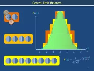
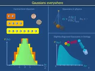
Variance: intuition • The variance of a random variable measures how far the distribution is spread out. • The variance is usually denoted by 2. • The square root of the variance is called the standard deviation. Larger variance Smaller variance ENGG2012B
Variance: definition • For a discrete random variable X with mean , the variance of X is defined as the expected deviation from the mean: • Useful trick in computing variance E[X2] is calledthe second momentof X ENGG2012B
General properties of variance • For any constant c, Var(c X) = c2 Var(X) • For any two independent r.v. X and Y, we have Var(X+Y) = Var(X) + Var(Y) (When X and Y are not independent, this may or may not be true.) ENGG2012B
SUM OF TWO INDEPENDENT R.V. ENGG2012B
Double up? • Compare the games on the left and right. + H H T H T T $0 $0 $0 H T H T H T $2 $1 $1 H T H H T T $4 $2 $2 H T H H T T $6 $3 $3 ENGG2012B
Sum of random variables • Let X1 and X2 be independent and identically distributed random variables, with pmf for i = 0,1,2,3,… • What is the distribution of X1 + X2? ENGG2012B
Enumerate all possibilities 1/2 1/4 1/8 1/64 1/32 1/16 X2=5 X2=0 X2=4 X2=1 X2=2 X2=3 X1=0 1/2 X1=1 1/4 1/8 X1=2 1/16 X1=3 X1=4 1/32 X1=5 1/64 We have use the assumption that X1 and X2 be independentwhen we fill in the probabilities in the table. ENGG2012B
Sum the entries for X1 + X2 = i 1/2 1/4 1/8 1/64 1/32 1/16 X2=5 X2=0 X2=4 X2=1 X2=2 X2=3 X1=0 1/2 X1=1 1/4 1/8 X1=2 1/16 X1=3 X1=4 1/32 X1=5 1/64 Pr(X1 + X2 =0) = 1/4 Pr(X1 + X2 =3) = 4/32 Pr(X1 + X2 =1) = 2/8 Pr(X1 + X2 =4) = 5/64 Pr(X1 + X2 =2) = 3/16 In general, Pr(X1 + X2 =i) = (i+1) / 2i+2 ENGG2012B
Using the summation sign, we can write For each non-negative integer i, // enumerate all possibilities // statistically independent // substitute the values for each r.v. ENGG2012B
Plot of the pmf of X1 + X2 for i=0,1,2,3… ENGG2012B
Convolution • The calculation of the pmf of the sum of two independent random variable is essentially a convolution operation. • Regard the pmf of a r. v. as a sequence of real numbers. Pmf of X1 : (0.5, 0.25, 0.125, 0.0625, …) Pmf of X2 : (0.5, 0.25, 0.125, 0.0625, …) (0.5, 0.25, 0.125, 0.0625, …) Pr(X1 + X2 =0) (…, 0.0625, 0.125, 0.25, 0.5) 0.25 ENGG2012B
Pmf of sum of two independent r.v. is the convolution of two pmf (0.5, 0.25, 0.125, 0.0625, …) 1/8+1/8=0.25 (0.5, 0.25, 0.125, 0.0625, …) 1/16+1/16+1/16 = 0.1875 (0.5, 0.25, 0.125, 0.0625, …) Pr(X1 + X2 =1) Pr(X1 + X2 =2) Pr(X1 + X2 =3) (…, 0.0625, 0.125, 0.25, 0.5) (…, 0.0625, 0.125, 0.25, 0.5) (…, 0.0625, 0.125, 0.25, 0.5) 1/32+1/32+1/32+1/32 = 0.125 ENGG2012B
Convolution in Matlab >> v = 2.^-(1:20) % the pmf of X, truncated after 20 >> f = conv(v,v) % take the convolution of v with itself >> stem(0: (length(f)-1),f) % stem plot ENGG2012B
POWER SERIES REPRESENTATION OF PMF ENGG2012B
Power series representation of pmf • A pmf can be represented by power series. • Suppose that the pmf of random variable X is f(i),for i=0,1,2,3,… • Define a power series • The coefficients are the values of function f. • The exponents of z are the values of X. • The power series is sometime called the generating function of f. ENGG2012B
Example • For the pmf f(i) = 1/2i+1 for i=0,1,2,3,… the power series representation is a geometric series: ENGG2012B
Calculating mean by power series • When evaluated at z=1, we get g(1)=1. • If we differentiate g(z) once and evaluate at z=1, we get the mean. ENGG2012B
Calculating variance by power series • If we differentiate twice and evaluate at z=1, we get the variance ENGG2012B
Example • For the pmf f(i) = 1/2i+1 for i=0,1,2,3,…the power series is g(z) = 1/(2-z). ENGG2012B
Power series is useful in calculating pmf of sum of two r.v. • Regard the pmf of a r. v. as a power series. • In the example of coin-tossing game, Pmf of X1 : g(z) = 0.5+ 0.25z + 0.125z2 + 0.0625z3 Pmf of X2 : h(z) = 0.5+ 0.25z + 0.125z2 + 0.0625z3 Pmf of X1 + X2 : g(z)h(z) = 0.25 + 0.25z + 0.1875z2 + 0.125z3 +… ENGG2012B
Calculation of pmf of sum of two independent r. v. • Convolution is just the product of two power series. • This is the same as the maxim“Convolution in time domain is equivalent to multiplication in frequency domain” For example: 0.5+ 0.25z +0.125z2 + 0.0625z3 + …) 1/16z2+1/16z2+1/16z2=0.1875z2 Pr(X1 + X2 =2)coeff. of z2 (…, 0.0625z3+ 0.125z2+ 0.25z + 0.5) ENGG2012B
2X vs X1+X2 • Compare the mean and variance of the two games. + H H T H T T $0 $0 $0 H T H T H T $2 $1 $1 H T H H T T $4 $2 $2 H T H H T T $6 $3 $3 ENGG2012B
2X vs X1+X2 • Suppose X, X1 and X2 are independent and identically distributed r.v. with pmf f(i) = 1/2i+1 for i=0,1,2,3,… • E[2X] = 2 E[X] =2, Var(2X) = 4Var(X) = 8. • E[X1 + X2] = E[X1] + E[X2] = 2, Var(X1 + X2) = Var(X1) + Var(X2) = 2+2=4. ENGG2012B
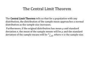
CENTRAL LIMIT THEOREM ENGG2012B
Pmf of X1 + X2 + X3 >> v = 2.^-(1:20) % the pmf of X , truncated after 20 >> f = conv(v,v) % take the convolution of v with itself >> f = conv(f,v) % take the convolution with v again >> stem(0: 30, f(1:31) ) % plot the first 31 numbers ENGG2012B