Pattern Matching Algorithms: An Overview

1. Pattern Matching Algorithms: An Overview Shoshana Neuburger The Graduate Center, CUNY 9/15/2009

2. Overview • Pattern Matching in 1D • Dictionary Matching • Pattern Matching in 2D • Indexing • Suffix Tree • Suffix Array • Research Directions

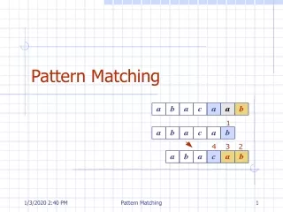
3. What is Pattern Matching? Given a pattern and text, find the pattern in the text.

4. What is Pattern Matching? • Σ is an alphabet. • Input: Text T = t1 t2 … tn Pattern P = p1 p2 … pm • Output: All i such that

5. Pattern Matching - Example Input: P=cagc = {a,g,c,t} T=acagcatcagcagctagcat • Output:{2,8,11} acagcatcagcagctagcat 1 2 3 4 5 6 78 …. 11

6. Pattern Matching Algorithms • Naïve Approach • Compare pattern to text at each location. • O(mn) time. • More efficient algorithms utilize information from previous comparisons.

7. Pattern Matching Algorithms • Linear time methods have two stages • preprocess pattern in O(m) time and space. • scan text in O(n) time and space. • Knuth, Morris, Pratt (1977): automata method • Boyer, Moore (1977): can be sublinear

8. KMP Automaton P = ababcb

9. Dictionary Matching • Σ is an alphabet. • Input: Text T = t1 t2 … tn Dictionary of patterns D = {P1, P2, …, Pk} All characters in patterns and text belong to Σ. • Output: All i, j such that where mj = |Pj|

10. Dictionary Matching Algorithms • Naïve Approach: • Use an efficient pattern matching algorithm for each pattern in the dictionary. • O(kn) time. More efficient algorithms process text once.

11. AC Automaton • Aho and Corasick extended the KMP automaton to dictionary matching • Preprocessing time: O(d) • Matching time: O(n log |Σ| +k). Independent of dictionary size!

12. AC Automaton D = {ab, ba, bab, babb, bb}

13. Dictionary Matching • KMP automaton does not depend on alphabet size while AC automaton does – branching. • Dori, Landau (2006): AC automaton is built in linear time for integer alphabets. • Breslauer (1995) eliminates log factor in text scanning stage.

14. Periodicity A crucial task in preprocessing stage of most pattern matching algorithms: computing periodicity. Many forms • failure table • witnesses

15. Periodicity • A periodic pattern can be superimposed on itself without mismatch before its midpoint. • Why is periodicity useful? Can quickly eliminate many candidates for pattern occurrence.

16. Periodicity Definition: • S is periodic if S = and is a proper suffix of . • S is periodic if its longest prefix that is also a suffix is at least half |S|. • The shortest period corresponds to the longest border.

17. Periodicity - Example S = abcabcabcab |S| = 11 • Longest border of S: b =abcabcab; |b| = 8 so S is periodic. • Shortest period of S: =abc = 3 so S is periodic.

18. Witnesses Popular paradigm in pattern matching: • find consistent candidates • verify candidates consistent candidates → verification is linear

19. Witnesses • Vishkin introduced the duel to choose between two candidates by checking the value of a witness. • Alphabet-independent method.

20. Witnesses Preprocess pattern: • Compute witness for each location of self-overlap. • Size of witness table: , if P is periodic, , otherwise.

21. Witnesses • WIT[i] = any k such that P[k] ≠ P[k-i+1]. • WIT[i] = 0, if there is no such k. k is a witness against i being a period of P. Example: Pattern Witness Table

22. Witnesses Let j>i. Candidates i and j are consistent if • they are sufficiently far from each other OR • WIT[j-i]=0.

23. Duel Scan text: • If pair of candidates is close and inconsistent, perform duel to eliminate one (or both). • Sufficient to identify pairwise consistent candidates: transitivity of consistent positions. P= T= witness i j a b ?

24. 2D Pattern Matching MRI • Σ is an alphabet. • Input: Text T [1… n, 1… n] Pattern P [1… m, 1… m] • Output: All (i, j) such that

25. 2D Pattern Matching - Example Input: Pattern = {A,B} Text Output:{ (1,4),(2,2),(4, 3)}

26. Bird / Baker • First linear-time 2D pattern matching algorithm. • View each pattern row as a metacharacter to linearize problem. • Convert 2D pattern matching to 1D.

27. Bird / Baker Preprocess pattern: • Name rows of pattern using AC automaton. • Using names, pattern has 1D representation. • Construct KMP automaton of pattern. Identical rows receive identical names.

28. Bird / Baker Scan text: • Name positions of text that match a row of pattern, using AC automaton within each row. • Run KMP on named columns of text. Since the 1D names are unique, only one name can be given to a text location.

29. Bird / Baker - Example Preprocess pattern: • Name rows of pattern using AC automaton. • Using names, pattern has 1D representation. • Construct KMP automaton of pattern.

30. Bird / Baker - Example Scan text: • Name positions of text that match a row of pattern, using AC automaton within each row. • Run KMP on named columns of text.

31. Bird / Baker • Complexity of Bird / Baker algorithm: time and space. • Alphabet-dependent. • Real-time since scans text characters once. • Can be used for dictionary matching: replace KMP with AC automaton.

32. 2D Witnesses • Amir et. al. – 2D witness table can be used for linear time and space alphabet-independent 2D matching. • The order of duels is significant. • Duels are performed in 2 waves over text.

33. Indexing • Index text • Suffix Tree • Suffix Array • Find pattern in O(m) time • Useful paradigm when text will be searched for several patterns.

34. banana$ anana$ nana$ ana$ na$ a$ $ n a b n a a a n n n a a a n a Suffix Trie T = banana$ suf7 suf1 suf2 suf3 suf4 suf5 suf6 suf7 $ $ suf6 $ suf5 $ suf4 $ suf3 $ suf2 $ suf1 • One leaf per suffix. • An edge represents one character. • Concatenation of edge-labels on the path from the root to leaf i spells the suffix that starts at position i.

35. banana$ anana$ nana$ ana$ na$ a$ $ na a banana$ na na$ na$ Suffix Tree T = banana$ [7,7] [3,4] suf1 suf2 suf3 suf4 suf5 suf6 suf7 $ [2,2] [1,7] [7,7] [3,4] [5,7] $ [7,7] suf6 suf1 [5,7] [7,7] $ suf3 suf5 $ suf2 suf4 • Compact representation of trie. • A node with one child is merged with its parent. • Up to n internal nodes. • O(n) space by using indices to label edges

36. Suffix Tree Construction • Naïve Approach: O(n2) time • Linear-time algorithms:

37. Suffix Tree Construction • Linear-time suffix tree construction algorithms rely on suffix links to facilitate traversal of tree. • A suffix link is a pointer from a node labeled xS to a node labeled S; x is a character and S a possibly empty substring. • Alphabet-dependent suffix links point from a node labeled S to a node labeled xS, for each character x.

38. Index of Patterns • Can answer Lowest Common Ancestor (LCA) queries in constant time if preprocess tree accordingly. • In suffix tree, LCA corresponds to Longest Common Prefix (LCP) of strings represented by leaves.

39. Index of Patterns To index several patterns: • Concatenate patterns with unique characters separating them and build suffix tree. Problem: inserts meaningless suffixes that span several patterns. OR • Build generalized suffix tree – single structure for suffixes of individual patterns. Can be constructed with Ukkonen’s algorithm.

40. Suffix Array • The Suffix Array stores lexicographic order of suffixes. • More space efficient than suffix tree. • Can locate all occurrences of a substring by binary search. • With Longest Common Prefix (LCP) array can perform even more efficient searches. • LCP array stores longest common prefix between two adjacent suffixes in suffix array.

41. Suffix Array Index Suffix Index Suffix LCP 1 mississippi 11 i 0 2 ississippi 8 ippi 1 3 ssissippi 5 issippi 1 4 sissippi 2 ississippi 4 5 issippi 1 mississippi 0 6 ssippi 10 pi 0 7 sippi 9 ppi 1 8 ippi 7 sippi 0 9 ppi 4 sissippi 2 10 pi 6 ssippi 1 11 i 3 ssissippi 3 sort suffixes alphabetically

42. 1 2 3 4 5 6 7 8 9 10 11 11 8 5 2 1 10 9 7 4 6 3 Index Suffix Suffix array T = mississippi LCP 0 1 1 4 0 0 1 0 2 1 3

43. Search in Suffix Array O(m log n): Idea: two binary searches- search for leftmost position of X- search for rightmost position of X In between are all suffixes that begin with X With LCP array: O(m + log n) search.

44. Suffix Array Construction • Naïve Approach: O(n2) time • Indirect Construction: • preorder traversal of suffix tree • LCA queries for LCP. Problem: does not achieve better space efficiency.

45. Suffix Array Construction • Direct construction algorithms: • LCP array construction: range-minima queries.

46. Compressed Indices Suffix Tree: O(n) words = O(n log n) bits Compressed suffix tree • Grossi and Vitter (2000) • O(n) space. • Sadakane (2007) • O(n log |Σ|) space. • Supports all suffix tree operations efficiently. • Slowdown of only polylog(n).

47. Compressed Indices Suffix array is an array of n indices, which is stored in: O(n) words = O(n log n) bits Compressed Suffix Array (CSA) Grossi and Vitter (2000) • O(n log |Σ|) bits • access time increased from O(1) to O(logε n) Sadakane (2003) • Pattern matching as efficient as in uncompressed SA. • O(n log H0) bits • Compressed self-index

48. Compressed Indices FM – index • Ferragina and Manzini (2005) • Self-indexing data structure • First compressed suffix array that respects the high-order empirical entropy • Size relative to compressed text length. • Improved by Navarro and Makinen (2007)

49. Dynamic Suffix Tree Dynamic Suffix Tree • Choi and Lam (1997) • Strings can be inserted or deleted efficiently. • Update time proportional to string inserted/deleted. • No edges labeled by a deleted string. • Two-way pointer for each edge, which can be done in space linear in the size of the tree.

50. Dynamic Suffix Array Dynamic Suffix Array • Recent work by Salson et. al. • Can update suffix array after construction if text changes. • More efficient than rebuilding suffix array. • Open problems: • Worst case O(n log n). • No online algorithm yet.