Download

1 / 29
380 likes | 917 Vues
Eigenvalues. The eigenvalue problem is to determine the nontrivial solutions of the equation Ax= x

E N D
Eigenvalues The eigenvalue problem is to determine the nontrivial solutions of the equation Ax= x where A is an n-by-n matrix, x is a length n column vector, and is a scalar. The n values of that satisfy the equation are the eigenvalues, and the corresponding values of x are the right eigenvectors. In MATLAB, the function eig solves for the eigenvalues , and optionally the eigenvectors x.
Eigenvalues If A is a square matrix of order (n x n) and I is the unit vector of the same order, then the matrix B = A - I Is called the characteristic matrix of A , being parameter, for example:
Eigenvalues A =
Eigenvalues The equation: B= (A-I)= 0 Is called characteristic equation of A and is in general an equation of the nth degree in . The n roots of this equation are called the characteristic roots ( or eigenvalues ) of A. For example, the characteristic equation of Matrix A is obtained by equating the determinant of B.
Eigenvalues That gives: • whose solution gives us • = 2, 2 2 , • stands as eigenvalues of A matrix
Eigenvalue Decomposition With the eigenvalues on the diagonal of a diagonal matrix and the corresponding eigenvectors forming the columns of a matrix V, we have: If V is nonsingular, this becomes the eigenvalue decomposition
Eigenvalue Decomposition A good example is provided by the coefficient matrix of the ordinary differential equation in the previous section. A = 0 -6 -1 6 2 -16 -5 20 -10
Eigenvalue Decomposition The statement lambda = eig(A) produces a column vector containing the eigenvalues. For this matrix, the eigenvalues are complex. lambda = -3.0710 -2.4645+17.6008i -2.4645-17.6008i
Eigenvalue Decomposition The real part of each of the eigenvalues is negative, so et approaches zero as t increases. The nonzero imaginary part of two of the eigenvalues, , contributes the oscillatory component, sint , to the solution of the differential equation.
Eigenvalue Decomposition With two output arguments, eig computes the eigenvectors and stores the eigenvalues in a diagonal matrix. [V,D] = eig(A) V = -0.8326 0.2003 - 0.1394i 0.2003 + 0.1394i -0.3553 -0.2110 - 0.6447i -0.2110 + 0.6447i -0.4248 -0.6930 -0.6930 D = -3.0710 0 0 0 -2.4645+17.6008i 0 0 0 -2.4645-17.6008
Eigenvalue Decomposition The first eigenvector is real and the other two vectors are complex conjugates of each other. All three vectors are normalized to have Euclidean length, norm(v,2), equal to one. The matrix V*D*inv(V), which can be written more succinctly as V*D/V, is within roundoff error of A. And, inv(V)*A*V, or V\A*V, is within roundoff error of D.
Defective Matrices Some matrices do not have an eigenvector decomposition. These matrices are defective, or not diagonalizable. For example, A = [ 6 12 19 -9 -20 -33 4 9 15 ]
Defective Matrices For this matrix [V,D] = eig(A) Produces V = -0.4741 -0.4082 -0.4082 0.8127 0.8165 0.8165 -0.3386 -0.4082 -0.4082 D = -1.0000 0 0 0 1.0000 0 0 0 1.0000 There is a double eigenvalue at = 1. The second and third columns of V are the same. For this matrix, a full set of linearly independent eigenvectors do not exist.
http://www.miislita.com/information-retrieval-tutorial/matrix-tutorial-3-eigenvalues-eigenvectors.html#dhttp://www.miislita.com/information-retrieval-tutorial/matrix-tutorial-3-eigenvalues-eigenvectors.html#d
The Eigenvalue Problem • Consider a scalar matrix Z, obtained by multiplying an identity matrix by a scalar; i.e., Z = c*I. Deducting this from a regular matrix A gives a new matrix A - c*I. A - Z = A - c*I. If its determinant is zero, |A - c*I| = 0 and A has been transformed into a singular matrix. The problem of transforming a regular matrix into a singular matrix is referred to as the eigenvalue problem.
Calculating Eigenvalues However, deducting c*I from A is equivalent to substracting a scalar c from the main diagonal of A. For the determinant of the new matrix to vanish the trace of A must be equal to the sum of specific values of c. For which values of c?
Calculating Eigenvalues • The polynomial expression we just obtained is called the characteristic equation and the c values are termed the latent roots or eigenvalues of matrix A. • Thus, deducting either c1 = 3 or c2 = 14 from the principal of A results in a matrix whose determinant vanishes (|A - c*I| = 0)
Calculating Eigenvalues In terms of the trace of A we can write: • c1/trace = 3/17 = 0.176 or 17.6%c2/trace = 14/17 = 0.824 or 82.4% Thus, c2 = 14 is the largest eigenvalue, accounting for more than 82% of the trace. The largest eigenvalue of a matrix is also called the principal eigenvalue.
Calculating Eigenvalues • Now that the eigenvalues are known, these are used to compute the latent vectors of matrix A. These are the so-called eigenvectors.
Eigenvectors A - ci*I Multiplying by a column vector Xi of same number of rows as A and setting the results to zero leads to : (A - ci*I)*Xi = 0 Thus, for every eigenvalue ci this equation constitutes a system of n simultaneous homogeneous equations, and every system of equations has an infinite number of solutions. Corresponding to every eigenvalue ci is a set of eigenvectors Xi, the number of eigenvectors in the set being infinite. Furthermore, eigenvectors that correspond to different eigenvalues are linearly independent from one another.
Properties of Eigenvalues and Eigenvectors • the absolute value of a determinant (|detA|) is the product of the absolute values of the eigenvalues of matrix A • c = 0 is an eigenvalue of A if A is a singular (noninvertible) matrix • If A is a nxn triangular matrix (upper triangular, lower triangular) or diagonal matrix , the eigenvalues of A are the diagonal entries of A. • A and its transpose matrix have same eigenvalues. • Eigenvalues of a symmetric matrix are all real.
Properties of Eigenvalues and Eigenvectors…..cont. • Eigenvectors of a symmetric matrix are orthogonal, but only for distinct eigenvalues. • The dominant or principal eigenvector of a matrix is an eigenvector corresponding to the eigenvalue of largest magnitude (for real numbers, largest absolute value) of that matrix. • For a transition matrix, the dominant eigenvalue is always 1. • The smallest eigenvalue of matrix A is the same as the inverse (reciprocal) of the largest eigenvalue of A-1; i.e. of the inverse of A.
In addition, it is confirmed that |c1|*|c2| = |3|*|14| = |42| = |detA|.
As show in earlier, plotting these vectors confirms that eigenvectors that correspond to different eigenvalues are linearly independent of one another. Note that each eigenvalue produces an infinite set of eigenvectors, all being multiples of a normalized vector. So, instead of plotting candidate eigenvectors for a given eigenvalue one could simply represent an entire set by its normalized eigenvector. This is done by rescaling coordinates; in this case, by taking coordinate ratios. In our example, the coordinates of these normalized eigenvectors are: (0.5, -1) for c1 = 3. (1, 0.2) for c2 = 14.
Concluding Remarks • Two of the eigenvalues are orthogonal. • Real part of eigenvalue is inverse of the time constant associated with principal mode of the system in time domain. • Imaginary part of eigenvalue gives angular frequency oscillation in frequency domain.