Download
1 / 58
620 likes | 863 Vues
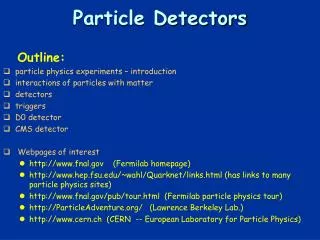
Particle Detectors. History of Instrumentation ↔ History of Particle Physics The ‘Real’ World of Particles Interaction of Particles with Matter Tracking Detectors, Calorimeters, Particle Identification Detector Systems. Summer Student Lectures 2011

E N D
Particle Detectors History of Instrumentation ↔ History of Particle Physics The ‘Real’ World of Particles Interaction of Particles with Matter Tracking Detectors, Calorimeters, Particle Identification Detector Systems Summer Student Lectures 2011 Werner Riegler, CERN, werner.riegler@cern.ch W. Riegler/CERN
Lectures are based on: C.W. Fabjan, Lectures on Particle Detectors P. Galison, Image and Logic C. Grupen, Particle Detectors G. Lutz, Semiconductor Radiation Detectors D. Green, The Physics of Particle Detectors W. Blum, W. Riegler, L. Rolandi, Particle Detection with Drift Chambers R. Wigmans, Calorimetry C. Joram, Summer Student Lectures 2003 C.D’Ambrosio et al., Postgraduate Lectures 2004, CERN O. Ullaland, Summer Student Lectures 2005 Particle Data Group Review Articles: http://pdg.web.cern.ch/pdg/ W. Riegler/CERN
History of Particle Physics 1895:X-rays, W.C. Röntgen 1896:Radioactivity, H. Becquerel 1899:Electron, J.J. Thomson 1911:Atomic Nucleus, E. Rutherford 1919:Atomic Transmutation, E. Rutherford 1920:Isotopes, E.W. Aston 1920-1930:Quantum Mechanics, Heisenberg, Schrödinger, Dirac 1932:Neutron, J. Chadwick 1932:Positron, C.D. Anderson 1937:Mesons, C.D. Anderson 1947:Muon, Pion, C. Powell 1947:Kaon, Rochester 1950:QED, Feynman, Schwinger, Tomonaga 1955:Antiproton, E. Segre 1956:Neutrino, Rheines etc. etc. etc. W. Riegler/CERN
History of Instrumentation 1906:Geiger Counter, H. Geiger, E. Rutherford 1910:Cloud Chamber, C.T.R. Wilson 1912:Tip Counter, H. Geiger 1928:Geiger-Müller Counter, W. Müller 1929:Coincidence Method, W. Bothe 1930:Emulsion, M. Blau 1940-1950:Scintillator, Photomultiplier 1952:Bubble Chamber, D. Glaser 1962:Spark Chamber 1968:Multi Wire Proportional Chamber, C. Charpak Etc. etc. etc. W. Riegler/CERN
On Tools and Instrumentation “New directions in science are launched by new tools much more often than by new concepts. The effect of a concept-driven revolution is to explain old things in new ways. The effect of a tool-driven revolution is to discover new things that have to be explained” From Freeman Dyson ‘Imagined Worlds’ W. Riegler/CERN
Physics Nobel Prices for Instrumentation 1927:C.T.R. Wilson, Cloud Chamber 1939:E. O. Lawrence, Cyclotron & Discoveries 1948:P.M.S. Blacket, Cloud Chamber & Discoveries 1950:C. Powell, Photographic Method & Discoveries 1954:Walter Bothe, Coincidence method & Discoveries 1960:Donald Glaser, Bubble Chamber 1968:L. Alvarez, Hydrogen Bubble Chamber & Discoveries 1992:Georges Charpak, Multi Wire Proportional Chamber • All Nobel Price Winners related to the Standard Model: 87 ! • (personal statistics by W. Riegler) • 31 for Standard Model Experiments 13 for Standard Model Instrumentation and Experiments 3 for Standard Model Instrumentation 21 for Standard Model Theory 9 for Quantum Mechanics Theory 9 for Quantum Mechanics Experiments 1 for Relativity • 56 for Experiments and instrumentation 31 for Theory W. Riegler/CERN
History of Instrumentation History of ‘Particle Detection’ Image Tradition: Cloud Chamber Emulsion Bubble Chamber Logic Tradition:Scintillator Geiger Counter Tip Counter Spark Counter Electronics Image: Wire Chambers Silicon Detectors … Peter Galison, Image and Logic A Material Culture of Microphysics W. Riegler/CERN
History of Instrumentation Image Detectors ‘Logic (electronics) Detectors ’ Bubble chamber photograph Early coincidence counting experiment W. Riegler/CERN
History of Instrumentation Both traditions combine into the ‘Electronics Image’ during the 1970ies Z-Event at UA1 / CERN W. Riegler/CERN
IMAGES W. Riegler/CERN
Cloud Chamber John Aitken, *1839, Scotland: Aitken was working on the meteorological question of cloud formation. It became evident that cloud droplets only form around condensation nuclei. Aitken built the ‘Dust Chamber’ to do controlled experiments on this topic. Saturated water vapor is mixed with dust. Expansion of the volume leads to super-saturation and condensation around the dust particles, producing clouds. From steam nozzles it was known and speculated that also electricity has a connection to cloud formation. Dust Chamber, Aitken 1888 W. Riegler/CERN
Cloud Chamber Charles Thomson Rees Wilson, * 1869, Scotland: Wilson was a meteorologist who was, among other things, interested in cloud formation initiated by electricity. In 1895 he arrived at the Cavendish Laboratory where J.J. Thompson, one of the chief proponents of the corpuscular nature of electricity, had studied the discharge of electricity through gases since 1886. Wilson used a ‘dust free’ chamber filled with saturated water vapor to study the cloud formation caused by ions present in the chamber. Cloud Chamber, Wilson 1895 W. Riegler/CERN
Cloud Chamber Conrad Röntgen discovered X-Rays in 1895. At the Cavendish Lab Thompson and Rutherford found that irradiating a gas with X-rays increased it’s conductivity suggesting that X-rays produced ions in the gas. Wilson used an X-Ray tube to irradiate his Chamber and found ‘a very great increase in the number of the drops’, confirming the hypothesis that ions are cloud formation nuclei. Radioactivity (‘Uranium Rays’) discovered by Becquerel in 1896. It produced the same effect in the cloud chamber. 1899 J.J. Thompson claimed that cathode rays are fundamental particles electron. Soon afterwards it was found that rays from radioactivity consist of alpha, beta and gamma rays (Rutherford). This tube is a glass bulb with positive and negative electrodes, evacuated of air, which displays a fluorescent glow when a high voltage current is passed though it. When he shielded the tube with heavy black cardboard, he found that a greenish fluorescent light could be seen from a platinobaium screen 9 feet away. W. Riegler/CERN
Cloud Chamber Using the cloud chamber Wilson also did rain experiments i.e. he studied the question on how the small droplets forming around the condensation nuclei are coalescing into rain drops. In 1908 Worthington published a book on ‘A Study of Splashes’ where he shows high speed photographs that exploited the light of sparks enduring only a few microseconds. This high-speed method offered Wilson the technical means to reveal the elementary processes of condensation and coalescence. With a bright lamp he started to see tracks even by eye ! By Spring 1911 Wilson had track photographs from from alpha rays, X-Rays and gamma rays. Worthington 1908 Early Alpha-Ray picture, Wilson 1912 W. Riegler/CERN
Cloud Chamber Wilson Cloud Chamber 1911 W. Riegler/CERN
Cloud Chamber X-rays, Wilson 1912 Alphas, Philipp 1926 W. Riegler/CERN
Cloud Chamber 1931 Blackett and Occhialini began work on a counter controlled cloud chamber for cosmic ray physics to observe selected rare events. The coincidence of two Geiger Müller tubes above and below the Cloud Chamber triggers the expansion of the volume and the subsequent Illumination for photography. W. Riegler/CERN
Cloud Chamber Magnetic field 15000 Gauss, chamber diameter 15cm. A 63 MeV positron passes through a 6mm lead plate, leaving the plate with energy 23MeV. The ionization of the particle, and its behaviour in passing through the foil are the same as those of an electron. Positron discovery, Carl Andersen 1933 W. Riegler/CERN
Cloud Chamber The picture shows and electron with 16.9 MeV initial energy. It spirals about 36 times in the magnetic field. At the end of the visible track the energy has decreased to 12.4 MeV. from the visible path length (1030cm) the energy loss by ionization is calculated to be 2.8MeV. The observed energy loss (4.5MeV) must therefore be cause in part by Bremsstrahlung. The curvature indeed shows sudden changes as can Most clearly be seen at about the seventeenth circle. Fast electron in a magnetic field at the Bevatron, 1940 W. Riegler/CERN
Cloud Chamber Taken at 3500m altitude in counter controlled cosmic ray Interactions. Nuclear disintegration, 1950 W. Riegler/CERN
Cloud Chamber Particle momenta are measured by the bending in the magnetic field. ‘ … The V0 particle originates in a nuclear Interaction outside the chamber and decays after traversing about one third of the chamber. The momenta of the secondary particles are 1.6+-0.3 BeV/c and the angle between them is 12 degrees … ‘ By looking at the specific ionization one can try to identify the particles and by assuming a two body decay on can find the mass of the V0. ‘… if the negative particle is a negative proton, the mass of the V0 particle is 2200 m, if it is a Pi or Mu Meson the V0 particle mass becomes about 1000m …’ Rochester and Wilson W. Riegler/CERN
Nuclear Emulsion Film played an important role in the discovery of radioactivity but was first seen as a means of studying radioactivity rather than photographing individual particles. Between 1923 and 1938 Marietta Blau pioneered the nuclear emulsion technique. E.g. Emulsions were exposed to cosmic rays at high altitude for a long time (months) and then analyzed under the microscope. In 1937, nuclear disintegrations from cosmic rays were observed in emulsions. The high density of film compared to the cloud chamber ‘gas’ made it easier to see energy loss and disintegrations. W. Riegler/CERN
Nuclear Emulsion In 1939 Cecil Powell called the emulsion ‘equivalent to a continuously sensitive high-pressure expansion chamber’. A result analog to the cloud chamber can be obtained with a picture 1000x smaller (emulsion density is about 1000x larger than gas at 1 atm). Due to the larger ‘stopping power’ of the emulsion, particle decays could be observed easier. Stacks of emulsion were called ‘emulsion chamber’. W. Riegler/CERN
Nuclear Emulsion Discovery of the Pion: The muon was discovered in the 1930ies and was first believed to be Yukawa’s meson that mediates the strong force. The long range of the muon was however causing contradictions with this hypothesis. In 1947, Powell et. al. discovered the Pion in Nuclear emulsions exposed to cosmic rays, and they showed that it decays to a muon and an unseen partner. The constant range of the decay muon indicated a two body decay of the pion. Discovery of muon and pion W. Riegler/CERN
Nuclear Emulsion Energy Loss is proportional to Z2 of the particle The cosmic ray composition was studied by putting detectors on balloons flying at high altitude. W. Riegler/CERN
Nuclear Emulsion First evidence of the decay of the Kaon into 3 Pions was found in 1949. Pion Kaon Pion Pion W. Riegler/CERN
Particles in the mid 50ies By 1959: 20 particles e- : fluorescent screen n : ionization chamber 7 Cloud Chamber: 6 Nuclear Emulsion: e+ +, - +, - anti-0 K0 + 0K+ ,K- - - 2 Bubble Chamber: 3 with Electronic techniques: 0 anti-n 0 anti-p 0 W. Riegler/CERN
Bubble Chamber In the early 1950ies Donald Glaser tried to build on the cloud chamber analogy: Instead of supersaturating a gas with a vapor one would superheat a liquid. A particle depositing energy along it’s path would then make the liquid boil and form bubbles along the track. In 1952 Glaser photographed first Bubble chamber tracks. Luis Alvarez was one of the main proponents of the bubble chamber. The size of the chambers grew quickly 1954: 2.5’’(6.4cm) 1954: 4’’ (10cm) 1956: 10’’ (25cm) 1959: 72’’ (183cm) 1963: 80’’ (203cm) 1973: 370cm W. Riegler/CERN
Bubble Chamber ‘old bubbles’ ‘new bubbles’ Unlike the Cloud Chamber, the Bubble Chamber could not be triggered, i.e. the bubble chamber had to be already in the superheated state when the particle was entering. It was therefore not useful for Cosmic Ray Physics, but as in the 50ies particle physics moved to accelerators it was possible to synchronize the chamber compression with the arrival of the beam. For data analysis one had to look through millions of pictures. W. Riegler/CERN
Bubble Chamber In the bubble chamber, with a density about 1000 times larger that the cloud chamber, the liquid acts as the target and the detecting medium. Figure: A propane chamber with a magnet discovered the S° in 1956. A 1300 MeV negative pion hits a proton to produce a neutral kaon and a S°, which decays into a L° and a photon. The latter converts into an electron-positron pair. W. Riegler/CERN
Bubble Chamber Discovery of the - in 1964 BNL, First Pictures 1963, 0.03s cycle W. Riegler/CERN
Bubble Chamber Gargamelle, a very large heavy-liquid (freon) chamber constructed at EcolePolytechnique in Paris, came to CERN in 1970. It was 2 m in diameter, 4 m long and filled with Freon at 20 atm. With a conventional magnet producing a field of almost 2 T, Gargamelle in 1973 was the tool that permitted the discovery of neutral currents. Can be seen outside the Microcosm Exhibition W. Riegler/CERN
Bubble Chamber The photograph of the event in the Brookhaven 7-foot bubble chamber which led to the discovery of the charmed baryon (a three-quark particle) is shown at left. A neutrino enters the picture from below (dashed line) and collides with a proton in the chamber's liquid. The collision produces five charged particles: A negative muon, three positive pions, and a negative pion and a neutral lambda. The lambda produces a characteristic 'V' when it decays into a proton and a pi-minus. The momenta and angles of the tracks together imply that the lambda and the four pions produced with it have come from the decay of a charmed sigma particle, with a mass of about 2.4 GeV. The detector began routine operations in 1974. The following year, the 7-foot chamber was used to discover the charmed baryon, a particle composed of three quarks, one of which was the "charmed" quark. W. Riegler/CERN
Bubble Chamber 3.7 meter hydrogen bubble chamber at CERN, equipped with the largest superconducting magnet in the world. During its working life from 1973 to 1984, the "Big European Bubble Chamber" (BEBC) took over 6 million photographs. Can be seen outside the Microcosm Exhibition W. Riegler/CERN
Bubble Chambers The excellent position (5m) resolution and the fact that target and detecting volume are the same (H chambers) makes the Bubble chamber almost unbeatable for reconstruction of complex decay modes. The drawback of the bubble chamber is the low rate capability (a few tens/ second). E.g. LHC 109 collisions/s. The fact that it cannot be triggered selectively means that every interaction must be photographed. Analyzing the millions of images by ‘operators’ was a quite laborious task. That’s why electronics detectors took over in the 70ties. W. Riegler/CERN
Logic and Electronics W. Riegler/CERN
Early Days of ‘Logic Detectors’ Electroscope: When the electroscope is given an electric charge the two ‘wings’ repel each other and stand apart. Radiation can ionize some of the air in the electroscope and allow the charge to leak away, as shown by the wings slowly coming back together. Scintillating Screen: Rutherford Experiment 1911, Zinc Sulfide screen was used as detector. If an alpha particle hits the screen, a flash can be seen through the microscope. Victor Hess discovered the Cosmic Rays by taking an electroscope on a Balloon W. Riegler/CERN
Geiger Rutherford In 1908, Rutherford and Geiger developed an electric device to measure alpha particles. The alpha particles ionize the gas, the electrons drift to the wire in the electric field and they multiply there, causing a large discharge which can be measured by an electroscope. The ‘random discharges’ in absence of alphas were interpreted as ‘instability’, so the device wasn’t used much. As an alternative, Geiger developed the tip counter, that became standard for radioactive experiments for a number of years. Rutherford and Geiger 1908 Tip counter, Geiger 1913 W. Riegler/CERN
Detector + Electronics 1925 ‘Über das Wesen des Compton Effekts’ W. Bothe, H. Geiger, April 1925 • Bohr, Kramers, Slater Theorie: • Energy is only conserved statistically • testing Compton effect ‘ Spitzenzähler ’ W. Riegler/CERN
Detector + Electronics 1925 ‘Über das Wesen des Compton Effekts’, W. Bothe, H. Geiger, April 1925 • ‘’Electronics’’: • Cylinders ‘P’ are on HV. • The needles of the counters are insulated and connected to electrometers. • Coincidence Photographs: • A light source is projecting both electrometers on a moving film role. • Discharges in the counters move the electrometers , which are recorded on the film. • The coincidences are observed by looking through many meters of film. W. Riegler/CERN
Detector + Electronics 1929 In 1928 Walther Müller started to study the sponteneous discharges systematically and found that they were actually caused by cosmic rays discovered by Victor Hess in 1911. By realizing that the wild discharges were not a problem of the counter, but were caused by cosmic rays, the Geiger-Müller counter went, without altering a single screw from a device with ‘fundametal limits’ to the most sensitive intrument for cosmic rays physics. ‘Zur Vereinfachung von Koinzidenzzählungen’ W. Bothe, November 1929 Coincidence circuit for 2 tubes W. Riegler/CERN
1930 - 1934 Cosmic ray telescope 1934 Rossi 1930: Coincidence circuit for n tubes W. Riegler/CERN
Geiger Counters By performing coincidences of Geiger Müller tubes e.g. the angular distribution of cosmic ray particles could be measured. W. Riegler/CERN
Scintillators, Cerenkov light, Photomultipliers In the late 1940ies, scintillation counters and Cerenkov counters exploded into use. Scintillation of materials on passage of particles was long known. By mid 1930 the bluish glow that accompanied the passage of radioactive particles through liquids was analyzed and largely explained (Cerenkov Radiation). Mainly the electronics revolution begun during the war initiated this development. High-gain photomultiplier tubes, amplifiers, scalers, pulse-height analyzers. W. Riegler/CERN
Antiproton One was looking for a negative particle with the mass of the proton. With a bending magnet, a certain particle momentum was selected (p=mv). Since Cerenkov radiation is only emitted if v>c/n, two Cerenkov counters (C1, C2) were set up to measure a velocity comparable with the proton mass. In addition the time of flight between S1 and S2 was required to be between 40 and 51ns, selecting the same mass. W. Riegler/CERN
Anti Neutrino Discovery 1959 Reines and Cowan experiment principle consisted in using a target made of around 400 liters of a mixture of water and cadmium chloride. The anti-neutrino coming from the nuclear reactor interacts with a proton of the target matter, giving a positron and a neutron. The positron annihilates with an electron of the surrounding material, giving two simultaneous photons and the neutron slows down until it is eventually captured by a cadmium nucleus, implying the emission of photons some 15 microseconds after those of the positron annihilation. + p n + e+ W. Riegler/CERN
Spark Counters The Spark Chamber was developed in the early 60ies. Schwartz, Steinberger and Lederman used it in discovery of the muon neutrino A charged particle traverses the detector and leaves an ionization trail. The scintillators trigger an HV pulse between the metal plates and sparks form in the place where the ionization took place. W. Riegler/CERN
Multi Wire Proportional Chamber Tube, Geiger- Müller, 1928 Multi Wire Geometry, in H. Friedmann 1949 G. Charpak 1968, Multi Wire Proportional Chamber, readout of individual wires and proportional mode working point. W. Riegler/CERN
MWPC Individual wire readout: A charged particle traversing the detector leaves a trail of electrons and ions. The wires are on positive HV. The electrons drift to the wires in the electric field and start to form an avalanche in the high electric field close to the wire. This induces a signal on the wire which can be read out by an amplifier. Measuring this drift time, i.e. the time between passage of the particle and the arrival time of the electrons at the wires, made this detector a precision positioning device. W. Riegler/CERN
The Electronic Image During the 1970ies, the Image and Logic devices merged into ‘Electronics Imaging Devices’ W. Riegler/CERN