Download
1 / 21
250 likes | 491 Vues
Cost Theory. EA Session 7 July 13, 2007 Prof. Samar K. Datta. Overview. Short run costs Long run costs & economies of scale Economies of scope & product transformation curve. SHORT RUN COSTS. Marginal Cost ( MC ) is the cost of expanding output by one unit => MC = dTC/dQ

E N D
Cost Theory EA Session 7 July 13, 2007 Prof. Samar K. Datta
Overview • Short run costs • Long run costs & economies of scale • Economies of scope & product transformation curve
SHORT RUN COSTS • Marginal Cost (MC) is the cost of expanding output by one unit => MC = dTC/dQ • Average Total Cost (ATC) is the cost per unit of output, or average fixed cost (AFC) plus average variable cost (AVC) => ATC = TC/Q = TFC/Q + TVC/Q = AFC + AVC • The relationship between the production function and cost can be exemplified by: • Increasing returns • With increasing returns, output is increasing relative to input and variable cost and total cost will fall relative to output. • Decreasing returns • With decreasing returns, output is decreasing relative to input and variable cost and total cost will rise relative to output.
The line drawn from the origin to the tangent of the variable cost curve: Its slope equals AVC The slope of a point on VC equals MC Therefore, MC = AVC at 7 units of output (point A) Cost Curves for a Firm TC P 400 VC 300 200 A 100 FC 0 1 2 3 4 5 6 7 8 9 10 11 12 13 Output
Unit Costs AFC falls continuously When MC < AVC or MC < ATC, AVC & ATC decrease When MC > AVC or MC > ATC, AVC & ATC increase When MC = AVC = ATC then AVC and ATC are at minimum Cost ($ per unit) 100 MC 75 50 ATC AVC 25 AFC 1 0 2 3 4 5 6 7 8 9 10 11 Output (units/yr.) Cost Curves for a Firm
Q1is an isoquant for output Q1. Isocost curve C0 shows all combinations of K and L that cost C0. K2 CO C1 C2 are three isocost lines A K1 Q1 K3 C0 C1 C2 L2 L1 L3 PRODUCING A GIVEN OUTPUT AT MINIMUM COST Capital per year Isocost C2 shows quantity Q1 can be produced with combination K2L2or K3L3. However, both of these are higher cost combinations than K1L1. Labor per year
E The long-run expansion path is drawn as before.. C Long-Run ExpansionPath A K2 Short-Run ExpansionPath P K1 Q2 Q1 L1 L2 L3 B D F THE INFLEXIBILITY OF SHORT-RUN PRODUCTION Capital per year Labor per year
RETURNS TO SCALE • Constant Returns to Scale • If input is doubled, output will double and average cost is constant at all levels of output. • Increasing Returns to Scale • If input is doubled, output will more than double and average cost decreases at all levels of output. • Decreasing Returns to Scale • If input is doubled, the increase in output is less than twice as large and average cost increases with output.
LMC LAC A LONG-RUN AVERAGE AND MARGINAL COST Cost ($ per unit of output Output
ECONOMIES AND DISECONOMIES OF SCALE • Measuring Economies of Scale • Therefore, the following is true: • EC < 1: MC < AC • economies of scale • EC = 1: MC = AC • constant economies of scale • EC > 1: MC > AC • diseconomies of scale
With many plant sizes with minimum SAC = $10 the LAC = LMC and is a straight line SAC1 SAC2 SAC3 SMC1 SMC2 SMC3 LAC = LMC $10 Q1 Q2 Q3 LONG-RUN COST WITH CONSTANT RETURNS TO SCALE Cost ($ per unit of output) Output
SAC1 LAC SAC3 SAC2 A $10 $8 B SMC1 If the output is Q1 a manager would chose the small plant SAC1 and SAC $8. Point B is on the LAC because it is a least cost plant for a given output. SMC3 LMC SMC2 Q1 LONG-RUN COST WITH ECONOMIESAND DISECONOMIES OF SCALE The long-run average cost curve is the envelope of the firm’s short-run average cost curves, assuming continually variable plant size. Cost ($ per unit of output The long-run cost curve is the dark blue portion of the SAC curve which represents the minimum cost for any level of output, assuming only three discrete plant sizes. Output
ECONOMIES OF SCOPE • Economies of scopeexist when the joint output of a single firm is greater than the output that could be achieved by two different firms each producing a single output. • Firms must choose how much of each to produce. • The alternative combinations can be illustrated using product transformation curves.
Each curve shows combinations of output with a given combination of L & K. O2 O1 illustrates a low level of output. O2 illustrates a higher level of output with two times as much labor and capital. O1 PRODUCT TRANSFORMATION CURVE Number of tractors Number of cars
ECONOMIES OF SCOPE • The degree of economies of scope measures the savings in cost and can be written: • C(Q1) is the cost of producing Q1 • C(Q2) is the cost of producing Q2 • C(Q1Q2) is the joint cost of producing both products • If SC > 0 --Economies of scope • If SC < 0 --Diseconomies of scope
DYNAMIC CHANGES IN COSTS –THE LEARNING CURVE (optional) • Thelearning curve measures the impact of worker’s experience on the costs of production. • It describes the relationship between a firm’s cumulative output and amount of inputs needed to produce a unit of output.
DYNAMIC CHANGES IN COSTS –THE LEARNING CURVE (optional) • The learning curve in the figure is based on the relationship:
DYNAMIC CHANGES IN COSTS –THE LEARNING CURVE (optional) • L equals A + B and this measures labor input to produce the first unit of output • Labor input remains constant as the cumulative level of output increases, so there is no learning
DYNAMIC CHANGES IN COSTS –THE LEARNING CURVE (optional) • L approaches A, and A represent minimum labor input/unit of output after all learning has taken place. • The more important the learning effect.
The chart shows a sharp drop in lots to a cumulative amount of 20, then small savings at higher levels. DYNAMIC CHANGES IN COSTS –THE LEARNING CURVE (optional) Hours of labor per machine lot 10 8 Doubling cumulative output causes a 20% reduction in the difference between the input required and minimum attainable input requirement. 6 4 2 Cumulative number of machine lots produced 0 10 20 30 40 50
Economies of Scale A B LAC1 Learning C LAC2 ECONOMIES OF SCALE VERSUS LEARNING (optional) Cost ($ per unit of output) Output