Download
1 / 45
450 likes | 529 Vues
Bisimulations as a Technique for State Space Reductions. symbolic state. represents a set of states. Abstract system. Original system. abstraction. Original property. Abstract property. P. P’. Safety:. The set of behaviors of the abstract system over-approximates

E N D
symbolic state represents a set of states Abstract system Original system abstraction Original property Abstract property P P’ Safety: The set of behaviors of the abstract system over-approximates the set of behaviors of the original system Abstraction: the key to scaling up
…, -2, 0, 2, 4, … Even …, -3, -1, 1, 3, … Odd …, -3, -2, -1 Neg 0 Zero Pos 1, 2, 3, … Data Abstraction vs. Predicate Abstraction • Data Abstraction • Abstraction proceeds component-wise, where variables are components x:int y:int
(0, 0) (1, 1) (-1, -1) true … (1, 2) false (-1, 3) (3, 2) … int * int Data Abstraction vs. Predicate Abstraction (Cont’d) • Predicate Abstraction • Use a boolean variable to hold the value of an associated predicate that expresses a relationship between variables predicate: x = y
An Example Init: x := 0; y := 0; z := 1; goto Body; Body: assert (z = 1); x := (x + 1); y := (y + 1); if (x = y) then Z1 else Z0; Z1: z := 1; goto Body; Z0: z := 0; goto Body; • x and y are unbounded • Data abstraction does not work in this case --- abstracting component-wise (per variable) cannot maintain the relationship between x and y • We will use predicate abstraction in this example
Predicate Abstraction Process • Add boolean variables to your program to represent current state of particular predicates • E.g., add a boolean variable [x=y] to represent whether the condition x=y holds or not • These boolean variables are updated whenever program statements update variables mentioned in predicates • E.g., add updates to [x=y] whenever x or y or assigned
p1: (x = 0) p2: (y = 0) p3: (x = (y + 1)) p4: (x = y) b1: [(x = 0)] b2: [(y = 0)] b3: [(x = (y + 1))] b4: [(x = y)] An Example Init: x := 0; y := 0; z := 1; goto Body; Body: assert (z = 1); x := (x + 1); y := (y + 1); if (x = y) then Z1 else Z0; Z1: z := 1; goto Body; Z0: z := 0; goto Body; • We will use the predicates listed below, and remove variables x and y since they are unbounded. • Don’t worry too much yet about how we arrive at this particular set of predicates; we will talk a little bit about that later Predicates Boolean Variables This is our new syntax for representing boolean variables that helps make the correspondence to the predicates clear
The statement to the left is replaced the statements below [(x=0)] := true; [(x=(y+1))] := if [$(y=0)] then false else top; [(x=y)] := if [$(y = 0)] then true else if ![$(y=0)] then false else top; Where: • [$P] = prev. value of [P] • top is a non-deterministic choice between true and false Make a more compact representation using a helper function H (following SLAM notation) [(x=0)] := true; [(x=y)] := H([$(y=0)], ![$(y=0)]); [(x=(y+1))] := H(false, [$(y=0)]); Where: true, if e1 H (e, e2) = false, if e2 top, otherwise { Transforming Programs An example of how to transform an assignment statement Predicates Assignment Statement x := 0; [(x = 0)] [(y = 0)] [(x = (y + 1))] [(x = y)]
simulates (n2,[x ! 2, y ! 2, z ! 0]) (n2,[x ! 3, y ! 3, z ! 0]) simulates (n2,[x ! 1, y ! 0, z ! 1]) does not simulates (n2,[x ! 3, y ! 3, z ! 1]) State Simulation Given a program abstracted by predicates E1, …, En, an abstract state simulates a concrete state if Ei holds on the concrete state iff the boolean variable [Ei] is true and remaining concrete vars and control points agree. Concrete Abstract (n2,[ [x=0] ! False, [y=0] ! False, [x=(y+1)] ! False, [x=y] ! True, z ! 0]) (n2,[ [x=0] ! False, [y=0] ! True, [x=(y+1)] ! True, [x=y] ! False, z ! 1])
Abstractions • Find reductions independent of the specification y. • Reduce K to K’ and construct a relation R such that for every (CTL) formulay • K, s ²y iff K’, s’ ²y where R(s, s’). • Note we do not transform y to y’.
Abstractions R s s’ K’ K
Bisimulations • K = (S, S0, R, AP, L) K’= (S’, S0’, R’, AP, L’) • Note K and K’ use the same set of atomic propositions AP. • Bµ S £ S’ is a bisimulation relation between K and K’ iff for every B(s, s’): • L(s) = L’(s’) (BSIM 1) • If R(s, s1) then there exists s1’ such that R’(s’, s1’) and B(s1, s1’). (BISIM 2) • If R(s’, s2’) then there exists s2 such that R(s, s2) and B(s2, s2’). (BISIM 3)
Bisimulations s s’ s1 K’ K
Bisimulations s s’ s1 s1’ K’ K
Bisimulations s s’ s2’ K’ K
Bisimulations s s’ s2 s1’ K’ K
Examples p q ….. p q p q p q
Examples p q ….. p q p q p q Unwinding preserves bisimulation
Examples p p q q q q r s r s r s
Examples p p q q q q r s r s r s
Examples p p q q q q r s r s r s
Examples p p q q q q r s r s r s
Examples p p q q q q r s r s r s
Examples p p q q q q r s r s r s
Examples p p q q q q r s r s r s
Bisimulations • K = (S, S0, R, AP, L) K’= (S’, S0’, R’, AP, L’) • K and K’ are bisimilar (bisimulation equivalent) iff there exists a bisimulation relation Bµ S £ S’ between K and K’ such that: • For each s0 in S0 there exists s0’ in S0’ such that B(s0 , s0’). • For each s0’ in S0’ there exists s0 in S0 such that B(s0 , s0’).
The Preservation Property. • K = (S, S0, R, AP, L) K’= (S’, S0’, R’, AP, L’) • Bµ S £ S’, a bisimulation. • Suppose B(s, s’). • FACT: For any CTL formula y (over AP), K, s ²y iff K’, s’ ²y. • If K’ is smaller than K this is worth something.
Bisimulation Quotients • Bisimulation equivalenec is an equivalence relation. • K = (S, S0, R, AP, L) • There is a maximal bisimulation Bµ S £ S. • Let R be this bisimulation. • [s] = {s’ j s R s’}. • R can be computed “easily”. • K’ = K / R is the bisimulation quotient of K.
Bisimulation Quotient • K = (S, S0, R, AP, L) • [s] = {s’ j s R s’}. • K’ = K / R = (S’, S’0, R’, AP,L’). • S’ = {[s] j s 2 S} • S’0 = {[s0] j s02 S0} • R’ = {([s], [s’]) j R(s1, s1’) for some s12 [s] and s1’ 2 [s’]} • L’([s]) = L(s).
Examples p q q r s r
Examples p q q r s r
Examples p q r s
Abstractions • Bisimulations don’t produce often large reduction. • Try notions such as simulations, data abstractions, symmetry reductions, partial order reductions etc. • Not all properties may be preserved. • They may not be preserved in a strong sense.
R G1 G2 x1 x2 a y1 Graph Simulation Definition Two edge-labeled graphs G1, G2 A simulation is a relation R between nodes: • if (x1, x2) R, and (x1,a,y1) G1, then exists (x2,a,y2) G2 (same label) s.t. (y1,y2) R a R y2 Note: if we insist that R be a function graph homeomorphism
Graph Bisimulation Definition Two edge-labeled graphs G1, G2 A bisimulation is a relation R between nodes s.t. both R and R-1 are simulations
Set Semantics for Semistructured Data Definition Two rooted graphs G1, G2 are equal if there exists a bisimulation R from G1 to G2 such that (root(G1), root(G2)) R • Notation: G1 G2 • For trees, this is precisely our earlier definition
Examples of Bisimilar Graphs a b b a = c c c a a = a a a a ...
Examples of non-Bisimilar Graphs • This is a simulation but not a bisimulation • Why ? • Notice: G1, G2 have the same sets of paths a a a G1= G2= b c b c
Examples of Simulation • Simulation acts like “subset” {a, b} {a, b, c} {a, b:{c}} {d, a:{e,f}, b:{c,g}} • Question: • if DB1 DB2 and DB2 DB1 then DB1 DB2 ? c a b a b d b a a b e c g f c
Answer if DB1 DB2 and DB2 DB1 then DB1 DB2 ? No. Here is a counter example: DB1 DB2 a a a b b DB1 DB2 and DB2 DB1 but NOT DB1 DB2
simulates simulates simulates simulates Path Simulation Intuition: every path in concrete system is simulated by a path in abstract system Concrete Abstract A concrete path s1, s2, … is simulated by an abstract path a1, a2, … if Sim(si,ai) for all i.
Infeasible path due to over-approximation. Computation Simulation Intuition: every path in concrete system is simulated by a path in abstract system Concrete Abstract There may be extra paths (termed “infeasible” paths) that are not present in the concrete system. These are due to the approximate nature of our computation with abstract tokens. Specifically, they arise from the over-approximations in test branching discussed previously.
Infeasible path due to over-approximation. Reflection of LTL Properties If there is a violating path in the concrete system, then there is a violating path in the abstract system, since the simulation property guarantees that each concrete trace has a corresponding trace in the abstract system. Technically, this means that properties are reflected by abstraction. Concrete Abstract If there is a violating path in the abstract system, then there is not necessarily a violating path in the concrete system, since the violating abstract trace may be an infeasible path due to over-approximation. Technically, this means that properties are not preserved by abstraction.
Facts About a (Bi)Simulation • The empty set is always a (bi)simulation • If R, R’ are (bi)simulations, so is R U R’ • Hence, there always exists a maximal (bi)simulation: • Checking if DB1=DB2: compute the maximal bisimulation R, then test (root(DB1),root(DB2)) in R
Computing a (Bi)Simulation • Computing the maximal (bi)simulation: • Start with R = nodes(G1) x nodes(G2) • While exists (x1, x2) R that violates the definition, remove (x1, x2) from R • This runs in polynomial time ! Better: • O((m+n)log(m+n)) for bisimulation • O(m n) for simulation • Compare to finding a graph homeomorphism ! NP Complete