Download
1 / 35
360 likes | 479 Vues
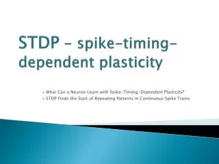
STDP Finds the Start of Repeating Patterns in Continuous Spike Trains. Timothee Masquelier, Rudy Guyonneau, Simon J. Thorpe. About Authors. Timothee Masquelier Computational Neuroscience Group, Universitat Pompeu Fabra, Barcelona, Spain

E N D
STDP Finds the Start ofRepeating Patterns in Continuous Spike Trains Timothee Masquelier, Rudy Guyonneau, Simon J. Thorpe
About Authors Timothee Masquelier Computational Neuroscience Group, Universitat Pompeu Fabra, Barcelona, Spain STDP in neural networks, implications for neural coding and information processing. Applications in the visual system for object and motion recognition Rudy Guyonneau The Brain and Cognition Research Center, Toulouse, France Biologically-inspired learning in asynchronously spiking neural networks Simon J. Thorpe Research Director CNRS,Toulouse, France Understanding the phenomenal processing speed achieved by the visual system
Discreet spike patterns learning* • A neuron is presented successively with discrete volleys of input spikes • STDP concentrates synaptic weights on afferents that consistently fire early • Postsynaptic spike latency decreases • Postsynaptic spike latency reaches a minimal and stable value Limitations: • Input spikes arrive in discrete volleys (spike waves) • Explicit time reference for coding allowing specification of latency • for afferents • Activity between volleys is assumed to be much weaker • Patterns presented in all volleys (no ‘distractor’ volleys) * Example: Masquelier T., Thorpe S.J. Unsupervised learning of visual features through STDP
Patterns learning with continuous spike firing • Afferents (sensory simulators) fire continuously with a constant population rate • Only a fraction of the recorded neurons are involved in the pattern • Pattern of spike repeats at irregular intervals, but is hidden within the variable background firing of the whole population • Nothing in terms of population firing rate characterizes the periods when the pattern is present • Nothing is unusual about the firing rates of the neurons involved in the pattern Detecting the pattern requires taking the spike times into account… • Is STDP is still able to find and learn spike patterns among the inputs? • What happens if pattern appears at unpredictable times separated by ‘distractor’ periods? • Is it OK to use the beginning of pattern as a time reference? • Does the postsynaptic latency still decrease with respect to the beginning of the pattern as time reference?
Simulation Environment • Single receiving STDP neuron with a 10ms membrane constant • Randomly generated ‘distractor’ spike trains (Poisson process with variable firing rates) 450s long • Arbitrary pattern inserted at various times (half of afferents left random mode for 50ms and adopted a precise firing pattern) • Same spike density of pattern and ‘distractor’ parts making pattern invisible in terms of firing rates • Unsupervised learning Afferents 1 STDP neuron
Distractor Spike Trains • Each afferent emits spikes independently using non-homogenous Poisson process: • Firing rate r varies between 0 and 90 Hz (dr = s.dt) • Max rate change sis selected to enable neuron going from 0 to 50 in 50ms • Random change is applied to s
Spatio-temporal spike patternNothing characterizes the averages in terms of firingrates. Detecting the pattern thus requires taking the spike times into account A repeating 50 ms long pattern that concerns 50 afferents among 100 Individual firing rates averaged over the whole period. Neurons involved in the pattern are shown in red The population-averaged firing rates over 10 ms time bins (membrane time constant of the neuron used in the simulations)
Additional Difficulties • Permanent 10 Hz Poissonian spontaneous activity • Arbitrary pattern inserted at various times (half of afferents left random mode for 50ms and adopted a precise firing pattern) • Same spike density of pattern and ‘distractor’ parts making pattern invisible in terms of firing rates • A 1ms jitter is added to the pattern Is it still possible to develop pattern selectivity in these conditions?
Happy Simulation Results One single Leaky Integrate-and-Fire neuron is perfectly able to solve the problem and learns to respond selectively to the start of the repeating pattern: • Implements STDP • Acts as coincidence detector ‘Successful’ simulation definition: • Postsynaptic latency inferior to 10 ms • Hit rate superior to 98% • No false alarms Observed in 96% of the cases (from 100 simulations) Limitation: Only excitation is considered, no inhibition in all these simulations
Spike Response Model • LIF is modeled using Gerstner’s Spike Response Model (SRM) • In SRM instead of solving the membrane potential diff. equation kernels are used to model the effect of presynaptic and postsynaptic spikes on the membrane potential • Refractoriness can be modelled as a combination of increased threshold, hyperpolarizing afterpotential, and reduced responsiveness after a spike, as observed in real neurons (Badel at al. 2008)
Spike Response Model • Membrane potential is given as: • t firing time of the last spike of the neuron • η response of the membrane to its own spike • k response of the neuron to the incoming short pulse • I(t) stimulating current • The next spike occurs if the membrane potential u hits a threshold in which case firing time of the last spike is updated
Connection between LIF and SRM It is possible to show that LIF is a special case of SRM • Take the differential equation of the LIF: • Integration of the differential equation for arbitrary input I(t), yields: • If we define k to be: it brings us to the general model equation
Spike Response Model • In case the input is generated by synaptic current pulses caused by presynaptic spike arrival the model can be rewritten as: =>
Spike Response Model • The kernel ε(t-tj) can be interpreted as the time course of a postsynaptic potential evoked by the firing of a presynaptic neuron j at time tj (EPSP in our case) = 10ms – membrane time constant = 2.5ms – synapse time constant Heaviside step function: K – multiplicative constant to scale the max value of the kernel to 1
Spike Response Model • The kernel ε(t-tj) can be interpreted as the time course of a postsynaptic potential evoked by the firing of a presynaptic neuron j at time tj (EPSP in our case) • The responsiveness ε to an input pulse depends on the time since last spike, because typically the effective membrane time constant after a spike is shorter, since many ion channels are open • The time course of the response is presented as a combination of exponentials with different time constants
Spike Response Model • The kernel η(t-ti) describes the standard form of an action potential of neuron i including the negative overshoot which typically follows a spike (after-potential) • T=500 - the threshold of the neuron • K1=2, K2=4 • Resting potential is zero • Both ε and η arerounded to zero when respectively t-tj and t-ti are greater than 7 * • wj – excitatory synaptic weights Positive pulse Negative spike after-potential
STDP Modification Function It was found that small learning rates led to more robust learning
Coincidence Detection • Coincidence detection relies on separate inputs converging on a common target • If each input neuron's EPSP is a sub-threshold for an action potential at target neuron, then it will not fire unless the n inputs from X1, X2, …, Xn are close together in time • For n=2, if the two inputs arrive too far apart, the depolarization of the first input may have time to drop significantly, preventing the membrane potential of the target neuron from reaching the action potential threshold
Simulation Data • At the beginning of the simulation the neuron is non-selective • Synaptic weights are all equal (w=0.475) • Neuron fires periodically, both inside and outside the pattern
After 70 Pattern Presentations and 700 Discharges • No false alarms • High hit rate • Neuron fires even twice when pattern is present • Chance determines which part(s) of the pattern the neuron becomes selective to
End of Simulation • The system is converged (by saturation) • Hit rate 99.1% with no false alarms • Postsynaptic spike latency reduction to 4ms (converged to saturation) • Fully specified neurons might have very low spontaneous rates • Higher spontaneous rates might characterize less well specified cells
Convergence by Saturation • All the spikes in the pattern that precede the postsynaptic spike already correspond to maximally potentiated synapses • All these spikes are needed to reach the threshold • Synapses corresponding to the spikes outside the pattern are fully depressed by STDP Bimodal Weight Distribution
Converged State Pattern boundaries Afferents out of pattern Afferents involved in pattern STDP has potentiated most of the synapses that correspond to the earliest spikes of the pattern Sudden increase in membrane potential corresponds to the white spikes cluster
Latency Reduction neuron is non-selective selectivity has emerged and STDP is ‘tracking back’ through the pattern the system has converged
Resistance to Degradation Additional batches of 100 simulations were performed to investigate the impact on successful performance of the following parameters: • Relative pattern frequency • Pattern duration • Amount of jitter • Proportion of afferents involved in the pattern • Initial weights • Proportion of missing spikes • Membrane constant
Pattern Frequency • Pattern frequency - sum of pattern durations over total duration ratio • Pattern needs to be consistently present for the STDP to establish selectivity. Later, longer distractor periods does not perturb the learning at all • Detection difficulty is related to the delay between two pattern presentations, not to the decrease in pattern duration Baseline condition – 0.25
Amount of Jitter For jitter larger than 3ms: • Spike coincidences are lost • STDP weight updates are inaccurate • Learning is impaired Millisecond spiking precision has been reported for brain Baseline condition – 1ms
Proportion of Afferents Involved inPattern Baseline condition – 1/2 • With fewer afferents involved in the pattern, it becomes harder to detect • Detected more than 50% with 1/3 afferents only => ‘developmental exuberance’ Developmental exuberance: Activity-driven mechanisms could select a small set of ‘interesting’ afferents among a much bigger set of initially connected afferents, probably specified genetically
Initial Weight Baseline condition – 0.475 For too many false discharges in a row the threshold may no longer be reachable as they lead to decrease of synaptic weights • High initial value for the weights increases the resistance to discharges outside the pattern • High initial weights also cause the neuron to discharge at a high rate at the beginning of the learning process
Proportion of Missing Spikes Baseline condition – 0% As expected number of successfully learned patterns decreases with the proportion of spikes deleted However the system is robust to spike deletion (82% success with a 10% deletion)
Conclusions • Main results previously obtained for STDP based learning with the highly simplified scheme of discrete spike volleys still stand in current more challenging continuous framework • It is not necessary to know a time reference in order to decode a temporal code, recurrent spike patterns in the inputs are enough, even embedded in equally dense ‘distractor’ spike trains • A neuron will gradually respond faster and faster when the pattern is presented, by potentiating synapses that correspond to the earliest spikes of the patterns, and depressing the others (substantial amount of information could be available very rapidly, in the very first spikes evoked by a stimuli)
Additional Observations • LIF neuron can never be selective to the whole pattern (membrane constant – 10ms, pattern duration – 50ms) • LIF is selective to ‘one coincidence’ of the pattern at a time, that is, selective to the nearly simultaneous arrival of certain earliest spikes, just as it occurs in one subdivision of the pattern (chance determines which one) • LIF can serve as ‘earliest predictor’ of the subsequent spike events: • Risk of triggering a false alarm • Benefit of being very reactive
Additional Observations – Cont. • If more than one repeating pattern is present in the input a postsynaptic neuron picks one (chance determines which one), and becomes selective to it and only to it • To learn the other patterns other neurons are needed. A competitive mechanism could ensure they optimally cover all the different patterns and avoid learning the same ones (inhibitory horizontal connections between neurons) • A long input pattern can be coded by the successive firings of several STDP neurons, each selective to a different part of the pattern • Further research is needed to evaluate this form of competitive network
Final Conclusion One single LIF neuron equipped with STDP is consistently able to detect one arbitrary repeating spatio-temporal spike pattern embedded in equally dense ‘distractor’ spike trains, which is a remarkable demonstration of the potential for such a scheme