Download
1 / 63
630 likes | 637 Vues
This lecture discusses lexical analysis, including identifying tokens in an input string, issues in lexical analysis, specifying lexers, and examples of regular expressions.

E N D
Lexical Analysis Lecture 2-4 Notes by G. Necula, with additions by P. Hilfinger Prof. Hilfinger CS 164 Lecture 2
Administrivia • Moving to 60 Evans on Wednesday • HW1 available • Pyth manual available on line. • Please log into your account and electronically register today. • Register your team with “make-team”. See class announcement page. Project #1 available Friday. • Use “submit hw1” to submit your homework this week. • Section 101 (9AM) is gone. Prof. Hilfinger CS 164 Lecture 2
Outline • Informal sketch of lexical analysis • Identifies tokens in input string • Issues in lexical analysis • Lookahead • Ambiguities • Specifying lexers • Regular expressions • Examples of regular expressions Prof. Hilfinger CS 164 Lecture 2
Source Tokens Interm. Language Parsing Today we start The Structure of a Compiler Lexical analysis Code Gen. Machine Code Optimization Prof. Hilfinger CS 164 Lecture 2
Lexical Analysis • What do we want to do? Example: if (i == j) z = 0; else z = 1; • The input is just a sequence of characters: \tif (i == j)\n\t\tz = 0;\n\telse\n\t\tz = 1; • Goal: Partition input string into substrings • And classify them according to their role Prof. Hilfinger CS 164 Lecture 2
What’s a Token? • Output of lexical analysis is a stream of tokens • A token is a syntactic category • In English: noun, verb, adjective, … • In a programming language: Identifier, Integer, Keyword, Whitespace, … • Parser relies on the token distinctions: • E.g., identifiers are treated differently than keywords Prof. Hilfinger CS 164 Lecture 2
Tokens • Tokens correspond to sets of strings: • Identifiers: strings of letters or digits, starting with a letter • Integers: non-empty strings of digits • Keywords: “else” or “if” or “begin” or … • Whitespace: non-empty sequences of blanks, newlines, and tabs • OpenPars: left-parentheses Prof. Hilfinger CS 164 Lecture 2
Lexical Analyzer: Implementation • An implementation must do two things: • Recognize substrings corresponding to tokens • Return: • The type or syntactic category of the token, • the value or lexeme of the token (the substring itself). Prof. Hilfinger CS 164 Lecture 2
Example • Our example again: \tif (i == j)\n\t\tz = 0;\n\telse\n\t\tz = 1; • Token-lexeme pairs returned by the lexer: • (Whitespace, “\t”) • (Keyword, “if”) • (OpenPar, “(“) • (Identifier, “i”) • (Relation, “==“) • (Identifier, “j”) • … Prof. Hilfinger CS 164 Lecture 2
Lexical Analyzer: Implementation • The lexer usually discards “uninteresting” tokens that don’t contribute to parsing. • Examples: Whitespace, Comments • Question: What happens if we remove all whitespace and all comments prior to lexing? Prof. Hilfinger CS 164 Lecture 2
Lookahead. • Two important points: • The goal is to partition the string. This is implemented by reading left-to-right, recognizing one token at a time • “Lookahead” may be required to decide where one token ends and the next token begins • Even our simple example has lookahead issues ivs. if =vs. == Prof. Hilfinger CS 164 Lecture 2
Next • We need • A way to describe the lexemes of each token • A way to resolve ambiguities • Is if two variables i and f? • Is ==two equal signs = =? Prof. Hilfinger CS 164 Lecture 2
Regular Languages • There are several formalisms for specifying tokens • Regular languages are the most popular • Simple and useful theory • Easy to understand • Efficient implementations Prof. Hilfinger CS 164 Lecture 2
Languages Def. Let S be a set of characters. A languageover S is a set of strings of characters drawn from S (S is called the alphabet ) Prof. Hilfinger CS 164 Lecture 2
Alphabet = English characters Language = English sentences Not every string on English characters is an English sentence Alphabet = ASCII Language = C programs Note: ASCII character set is different from English character set Examples of Languages Prof. Hilfinger CS 164 Lecture 2
Notation • Languages are sets of strings. • Need some notation for specifying which sets we want • For lexical analysis we care about regular languages, which can be described using regular expressions. Prof. Hilfinger CS 164 Lecture 2
Regular Expressions and Regular Languages • Each regular expression is a notation for a regular language (a set of words) • If A is a regular expression then we write L(A) to refer to the language denoted by A Prof. Hilfinger CS 164 Lecture 2
Atomic Regular Expressions • Single character: ‘c’ L(‘c’) = { “c” } (for any c ) • Concatenation: AB(where A and B are reg. exp.) L(AB) = { ab | a L(A) and b L(B) } • Example: L(‘i’ ‘f’) = { “if” } (we will abbreviate ‘i’ ‘f’ as ‘if’ ) Prof. Hilfinger CS 164 Lecture 2
Compound Regular Expressions • Union L(A | B) = L(A) L(B) = { s | s L(A) or s L(B) } • Examples: ‘if’ | ‘then‘ | ‘else’ = { “if”, “then”, “else”} ‘0’ | ‘1’ | … | ‘9’ = { “0”, “1”, …, “9” } (note the … are just an abbreviation) • Another example: L((‘0’ | ‘1’) (‘0’ | ‘1’)) = { “00”, “01”, “10”, “11” } Prof. Hilfinger CS 164 Lecture 2
More Compound Regular Expressions • So far we do not have a notation for infinite languages • Iteration: A* L(A*) = { “” } | L(A) | L(AA) | L(AAA) | … • Examples: ‘0’* = { “”, “0”, “00”, “000”, …} ‘1’ ‘0’* = { strings starting with 1 and followed by 0’s } • Epsilon: L() = { “” } Prof. Hilfinger CS 164 Lecture 2
Example: Keyword • Keyword: “else” or “if” or “begin” or … ‘else’ | ‘if’ | ‘begin’ | … (‘else’ abbreviates ‘e’ ‘l’ ‘s’ ‘e’ ) Prof. Hilfinger CS 164 Lecture 2
Example: Integers Integer: a non-empty string of digits digit = ‘0’ | ‘1’ | ‘2’ | ‘3’ | ‘4’ | ‘5’ | ‘6’ | ‘7’ | ‘8’ | ‘9’ number = digit digit* Abbreviation: A+ = A A* Prof. Hilfinger CS 164 Lecture 2
Example: Identifier Identifier: strings of letters or digits, starting with a letter letter = ‘A’ | … | ‘Z’ | ‘a’ | … | ‘z’ identifier = letter (letter | digit) * Is (letter* | digit*) the same as (letter | digit) * ? Prof. Hilfinger CS 164 Lecture 2
Example: Whitespace Whitespace: a non-empty sequence of blanks, newlines, and tabs (‘ ‘ | ‘\t’ | ‘\n’)+ (Can you spot a subtle omission?) Prof. Hilfinger CS 164 Lecture 2
Example: Phone Numbers • Regular expressions are all around you! • Consider (510) 643-1481 = { 0, 1, 2, 3, …, 9, (, ), - } area = digit3 exchange = digit3 phone = digit4 number = ‘(‘ area ‘)’ exchange ‘-’ phone Prof. Hilfinger CS 164 Lecture 2
Example: Email Addresses • Consider necula@cs.berkeley.edu = letters [ { ., @ } name = letter+ address = name ‘@’ name (‘.’ name)* Prof. Hilfinger CS 164 Lecture 2
Summary • Regular expressions describe many useful languages • Next: Given a string s and a R.E. R, is s L( R ) ? • But a yes/no answer is not enough ! • Instead: partition the input into lexemes • We will adapt regular expressions to this goal Prof. Hilfinger CS 164 Lecture 2
Next: Outline • Specifying lexical structure using regular expressions • Finite automata • Deterministic Finite Automata (DFAs) • Non-deterministic Finite Automata (NFAs) • Implementation of regular expressions RegExp => NFA => DFA => Tables Prof. Hilfinger CS 164 Lecture 2
Regular Expressions => Lexical Spec. (1) • Select a set of tokens • Number, Keyword, Identifier, ... • Write a R.E. for the lexemes of each token • Number = digit+ • Keyword = ‘if’ | ‘else’ | … • Identifier = letter (letter | digit)* • OpenPar = ‘(‘ • … Prof. Hilfinger CS 164 Lecture 2
Regular Expressions => Lexical Spec. (2) • Construct R, matching all lexemes for all tokens R = Keyword | Identifier | Number | … = R1 | R2 | R3 | … Facts: If s L(R) then s is a lexeme • Furthermore s L(Ri) for some “i” • This “i” determines the token that is reported Prof. Hilfinger CS 164 Lecture 2
Regular Expressions => Lexical Spec. (3) • Let the input be x1…xn (x1 ... xnare characters in the language alphabet) • For 1 i n check x1…xi L(R) ? • It must be that x1…xi L(Rj) for some i and j • Remove x1…xi from input and go to (4) Prof. Hilfinger CS 164 Lecture 2
Lexing Example R = Whitespace | Integer | Identifier | ‘+’ • Parse “f+3 +g” • “f” matches R, more precisely Identifier • “+“ matches R, more precisely ‘+’ • … • The token-lexeme pairs are (Identifier, “f”), (‘+’, “+”), (Integer, “3”) (Whitespace, “ “), (‘+’, “+”), (Identifier, “g”) • We would like to drop the Whitespace tokens • after matching Whitespace, continue matching Prof. Hilfinger CS 164 Lecture 2
Ambiguities (1) • There are ambiguities in the algorithm • Example: R = Whitespace | Integer | Identifier | ‘+’ • Parse “foo+3” • “f” matches R, more precisely Identifier • But also “fo” matches R, and “foo”, but not “foo+” • How much input is used? What if • x1…xi L(R) and also x1…xK L(R) • “Maximal munch” rule: Pick the longest possible substring that matches R Prof. Hilfinger CS 164 Lecture 2
More Ambiguities R = Whitespace | ‘new’ | Integer | Identifier • Parse “newfoo” • “new” matches R, more precisely ‘new’ • but also Identifier, which one do we pick? • In general, if x1…xi L(Rj) and x1…xi L(Rk) • Rule: use rule listed first (j if j < k) • We must list ‘new’ before Identifier Prof. Hilfinger CS 164 Lecture 2
Error Handling R = Whitespace | Integer | Identifier | ‘+’ • Parse “=56” • No prefix matches R: not “=“, nor “=5”, nor “=56” • Problem: Can’t just get stuck … • Solution: • Add a rule matching all “bad” strings; and put it last • Lexer tools allow the writing of: R = R1 | ... | Rn | Error • Token Error matches if nothing else matches Prof. Hilfinger CS 164 Lecture 2
Summary • Regular expressions provide a concise notation for string patterns • Use in lexical analysis requires small extensions • To resolve ambiguities • To handle errors • Good algorithms known (next) • Require only single pass over the input • Few operations per character (table lookup) Prof. Hilfinger CS 164 Lecture 2
Finite Automata • Regular expressions = specification • Finite automata = implementation • A finite automaton consists of • An input alphabet • A set of states S • A start state n • A set of accepting states F S • A set of transitions state input state Prof. Hilfinger CS 164 Lecture 2
Finite Automata • Transition s1as2 • Is read In state s1 on input “a” go to state s2 • If end of input • If in accepting state => accept, othewise => reject • If no transition possible => reject Prof. Hilfinger CS 164 Lecture 2
a Finite Automata State Graphs • A state • The start state • An accepting state • A transition Prof. Hilfinger CS 164 Lecture 2
1 A Simple Example • A finite automaton that accepts only “1” • A finite automaton accepts a string if we can follow transitions labeled with the characters in the string from the start to some accepting state Prof. Hilfinger CS 164 Lecture 2
1 0 Another Simple Example • A finite automaton accepting any number of 1’s followed by a single 0 • Alphabet: {0,1} • Check that “1110” is accepted but “110…” is not Prof. Hilfinger CS 164 Lecture 2
1 0 0 0 1 1 And Another Example • Alphabet {0,1} • What language does this recognize? Prof. Hilfinger CS 164 Lecture 2
1 1 And Another Example • Alphabet still { 0, 1 } • The operation of the automaton is not completely defined by the input • On input “11” the automaton could be in either state Prof. Hilfinger CS 164 Lecture 2
Epsilon Moves • Another kind of transition: -moves A B • Machine can move from state A to state B without reading input Prof. Hilfinger CS 164 Lecture 2
Deterministic and Nondeterministic Automata • Deterministic Finite Automata (DFA) • One transition per input per state • No -moves • Nondeterministic Finite Automata (NFA) • Can have multiple transitions for one input in a given state • Can have -moves • Finite automata have finite memory • Need only to encode the current state Prof. Hilfinger CS 164 Lecture 2
Execution of Finite Automata • A DFA can take only one path through the state graph • Completely determined by input • NFAs can choose • Whether to make -moves • Which of multiple transitions for a single input to take Prof. Hilfinger CS 164 Lecture 2
1 0 0 1 Acceptance of NFAs • An NFA can get into multiple states • Input: 1 0 1 • Rule: NFA accepts if it can get in a final state Prof. Hilfinger CS 164 Lecture 2
NFA vs. DFA (1) • NFAs and DFAs recognize the same set of languages (regular languages) • DFAs are easier to implement • There are no choices to consider Prof. Hilfinger CS 164 Lecture 2
0 0 0 1 1 0 0 0 1 1 NFA vs. DFA (2) • For a given language the NFA can be simpler than the DFA NFA DFA • DFA can be exponentially larger than NFA Prof. Hilfinger CS 164 Lecture 2
Regular Expressions to Finite Automata • High-level sketch NFA Regular expressions DFA Lexical Specification Table-driven Implementation of DFA Prof. Hilfinger CS 164 Lecture 2