Download
1 / 64
650 likes | 843 Vues
3D From 2D. Image Processing Seminar. Presented by: Eli Arbel. Topics Covered. Inferring 3D surfaces from 2D contours using symmetry From a single view Using symmetry to enhance structure from motion methods Sequence of images. Inferring 3D surfaces from 2D contours using symmetry.

E N D
3D From 2D Image Processing Seminar Presented by: Eli Arbel
Topics Covered • Inferring 3D surfaces from 2D contours using symmetry • From a single view • Using symmetry to enhance structure from motion methods • Sequence of images
The challenges • Recover orientations of 3D surfaces projected on 2D image. • Ambiguity - Infinite number of interpretations for a single image • Cannot be done without some assumptions
The challenges, cont`d • Still, humans are able to perceive 3D surfaces in a single image…
Monocular Cues • Shading • Reflectance properties of the surface, light sources • Texture • Prior knowledge required • Contour lines • Give shape information near the contours only • What about conflicts ?
The method • Based on symmetries in the scene to infer surface orientation • Assumes orthographic projection • Also considers interaction between surfaces
Curves of symmetry Lines of symmetry Axis of symmetry Symmetries • Defined as pointwise correspondence between two curves
Symmetries – Cont’d • Parallel symmetry: • Skew symmetry:
Qualitative inferences from symmetries • Symmetries can be major source of information for extracting shape from contour • Can give constraints on interpretations of single surfaces Definition: General Viewpoint A scene is said to be imaged from general viewpoint if its perceptual properties are preserved under slight variations of the viewing direction • In particular: straightness, parallelity and curves symmetry
Qualitative inferences – Case I • Case I: one skew symmetry covers the entire boundary of the surface • That kind of contour – if bounded by non-limb edges – must be planar under the assumption of general viewpoint Definition: Limb edges points on the surface whose normal is orthogonal to the viewing direction • Non-limb edges: wireframes
Qualitative inferences – Case I Proof: • Parallel lines in the image plane must a projection of parallel lines in 3D space. Thus, the symmetry lines are parallel in 3D. • Axis of the skew symmetry must be a projection of a straight line. • The axis of symmetry is obtained by connecting the midpoints of the symmetry lines From 1,2 and 3 above, the 3D contour must be planar.
Qualitative inferences – Case II • Case II: Boundary is covered by two symmetries, at least one of them must be parallel symmetry • Figures belong to case II give us the most information about surface shape
Non ZGC ZGC Qualitative inferences – Case II Definition: Zero Gaussian Curvature (ZGC) Surface Surface in which the product of the minimum and maximum curvature is zero everywhere
Qualitative inferences – Case II • If the surface generates one parallel symmetry and one skew symmetry with straight curves of skew symmetry which are also the lines of symmetry for parallel symmetry, then the surface must be ZGC surface. • Assuming general viewpoint and no surface variations that do not produce edges in the image plane • Can be proved…
Qualitative inferences – Case III • Case III: Includes all remaining cases. • Contours satisfy specific properties • Figures which have some missing boundaries • All other cases.
Recovering Surface Orientations • Reminder: In order to recover a 3D surface from 2D projection, we need to find the orientation (normal) of each point of the surface • Orientations of a surface can be recovered using constraints system derived from symmetries in the image • We will focus on ZGC surfaces.The presence of ZGC surfaces is indicated by observing the properties given above.
Some Math… • Parametric representation of curves: S(r) = (x(r), y(r)) in 2D S(r) = (x(r), y(r), z(r)) in 3D
Some More Math... • Parametric representation of a surface: X(u,v) = (x(u,v), y(u,v), z(u,v))
Plane can be rewritten as , and so its normal vector: or (p,q,1) where and And a little more... • Gradient Space: • Given a plane, , its normal N is given by the vector (A, B, C) - the gradient vector. • (p,q) defines 2D space such that every point at this space corresponds to the normal of a plane in 3D
Rulings • Note: orientations of a ZGC surface does not change along a ruling. One Last Thing... Definition: Rulings the lines connecting corresponding points of two curves forming parallel symmetry. (correspondence is determined by the tangent of the curves)
Two surfaces: Xi(u,v), i=1,2 X2 N2 Intersection curve: Tangent vector: N1 Normal vectors: Ni(s)=(pi(s), qi(s), 1), i=1,2 (in p-q space) X1 Since is on the tangent planes of both X1 and X2, it’s orthogonal to both N1(s) and N2(s). That is: Curved Shared Boundary Constraint - CSBC • This constraint relates the orientations of two surfaces of opposite sides of an edge
Note that can be extracted from the image CSBC – cont’d • A stronger constraint can be obtained if we assume that the intersection curve is planar. • Let N1=(pc,qc,1) be the normal of the plane on which lies on. From this constraint: we get: X2 X1
Let X(u,v)=(x(u,v), y(u,v), z(u,v)) be a parametric representation of a surface, and v be along the direction of the minimum curvature (rulings for ZGC surfaces). • ISC intuitive description: as we move along the u parameter (axis of symmetry), the surface orientation should move in p-q plane in a direction orthogonal to the direction of the rulings. q Ri Ri • • i+1 i p • • (pi+1,qi+1) (pi,qi) Inner Surface Constraint - ISC • This constraint restricts the relative orientations of neighboring points within a surface, using the image of the surface’s rulings.
According to ISC, the following equation should hold: q Ri p • • (pi+1,qi+1) (pi,qi) ISC – cont’d • The change in the surface’s orientation when moving from point i to point i+1 in the p-q space is given by the vector (pi+1-pi, qi+1-qi) • Let (xi, yi) be the direction of the ruling Ri. • Again, (xi, yi) can be computed directly from the image
Cut along Curves of maximum curvature ? OC perception Preferred perception Orthogonality Constraint - OC • This constraint is derived from the assumption of orthogonality between the axis of parallel symmetry and the lines of symmetry. • For ZGC surfaces, this constrained implies that the cross section must be along the lines of maximum curvature. However, in general, this conflicts with our drive to perceive the cross section as being planar.
A is the tangent vector of the axis of symmetry A B B is the tangent vector of the ruling Let N=(p,q,1) be the normal of the tangent plane at that point. Since A and B are on the tangent plane of the surface, they can be represented as: From the orthogonality constraint, we get or: OC – cont’d Given a ZGC surface:
Combining the Constraints • In order to recover 3D surface from its 2D projection, we need to know the orientation at each point in the surface. • For a ZGC surface ,the orientation along the ruling is constant, thus it is sufficient to find the orientation of a single point on the ruling. • These leaves us with computing the orientation of points along the axis of symmetry
Equations: n CSBC: n-1 ISC: n OC: • We have 3n-1 constraints equation producing 2n+2 unknowns. • For n > 3, the system is over constrained Combining the Constraints – cont’d • Suppose the surface orientation is to be computed for n points:
Combining the Constraints – cont’d • Because the system is over constrained, it may be impossible to find interpretation for the contours such that all the constraints are obeyed by the surface. • OC and the planarity of the cross section assumed by CSBC are usually in conflict. • However, there are cases where these set of constraints may give a unique answer or even leave one degree of freedom unconstrained.
Recoverable Surfaces Circular Cones: • A circular cone in linear straight homogenous generalized cylinder, whose cross section is a circle. • These are the only surfaces that have a unique solution to the three constraints.
Recoverable Surfaces – cont’d Cylindrical surfaces • A cylindrical surface is a ZGC surface for which rulings are parallel to each other in 3D. • With these kind of surfaces, we have one degree of freedom – qc in CSBC.
Recoverable Surfaces – cont’d General ZGC surfaces • For general ZGC surfaces, the three constraints cannot be satisfied exactly. • In most cases, planarity assumption is stronger then the orthogonality assumption. • The solution is to maximize the orthogonality while keeping CSBC and ISC satisfied exactly. • Again, the degree of freedom is in the orientation of the cross section plane, namely (pc,qc).
Estimating (pc,qc) • The method is based on observations of human perception preferences. In particular: • We prefer compact shapes. • We prefer medium slant to very high or very low slant. • We have a large range of uncertainty for the perceived slants.
Estimating (pc,qc) – cont’d • An ellipse-fitting process is applied on the top surface to approximate an ellipse to the cross section.
Estimating (pc,qc) – cont’d • After the ellipse is fitted, the orientation of the circle that would project as the fitted ellipse is found. • This orientation becomes (pc,qc). • A final update of qc is performed to reflect the bias humans have in orienting the cross section toward 45º. • The above technique was developed as a consequence of experimental results with humans. • It was found that humans estimation of top planes slants is imprecise with an average standard deviation of 8º. • The average of the differences between the algorithm estimation and human estimation are 6º.
Testing The Algorithm • The inputs to the program are collection of curves grouped into closed regions using continuity • Each closed region is considered to be a surface • Each curve in the region is checked for parallel symmetry against every other curve in the region. • Two curves are considered to be parallel symmetric if they return low symmetry error which is defined as:
Testing The Algorithm – cont’d • Surfaces containing parallel symmetry are treated as curved and others as planar. • For curved surfaces, the curves joining parallel symmetric curves are checked if they are straight, which confirms that the surface is ZGC. • For each surface the orientation of the planar cross section (pc,qc) is computed. • Orientation at each point (pi,qi) on the surface is computed using ISC and CSBC constraints.
Using Bilateral Symmetry ToImprove 3D Reconstruction From Image Sequences
Introduction • Structure from motion methods • Like stereo with single camera • Static scene • Sequence of images, each one is a different view of the object • Reconstruction based on features • Like other methods, sensitive to noise
Noisy Projections • Noise can be present in the 2D projections of the scene due to measurements deviations, motion of the camera, etc.. • 3D mirror symmetry is one of the most common symmetry in our environment • In case the reconstructed object is known to be mirror symmetric, a symmetrization procedure can be applied on the noisy projections to enhance reconstruction of the 3D object
The Framework • Apply symmetrization procedure to the 2D data with respect to the 3D symmetry • Reconstruct the object using any structure from motion method • Given the 3D configuration of stage 2, find the closest mirror-symmetric configuration to it
Definition: Symmetry Distance Let be a mirror-symmetric configuration derived from . The symmetry distance is the quantity: 3D symmetrization • Consider a 3D configuration of points • If the configuration is from 3D mirror-symmetric object then for every point there exist a point which is its counterpart under reflection
º • º 2. Reflect all points across a randomly chosen mirror plane, obtaining the points . • • º º º 3. Find the optimal rotation and translation which minimizes the sum of squared distances between the original points and the reflected points • º • • º • º 4. Average each original point with its reflected point obtaining the point . The points are mirror symmetric. • 3D Symmetrization Algorithm • Given a configuration of points in : 1. Divide the points into sets of one or two points. For instance: {P0,P0}, {P1,P3}, {P2,P2}. This defines a matching on the points. 5. Evaluate the Symmetry Distance 6. Minimize the Symmetry Distance by repeating steps 1-5 with all possible divisions of points to sets.
Graph Matching rank 1 rank 3 rank 4 • • • • • • • • • • • Complexity Of Matching • Matching of feature points is of exponential complexity • However, by constraining the search space of all possible matches, complexity can be greatly reduced • Is it Sufficient ? • We might need to consider higher order connectivity as well (maximal…)