Download
1 / 21
220 likes | 373 Vues
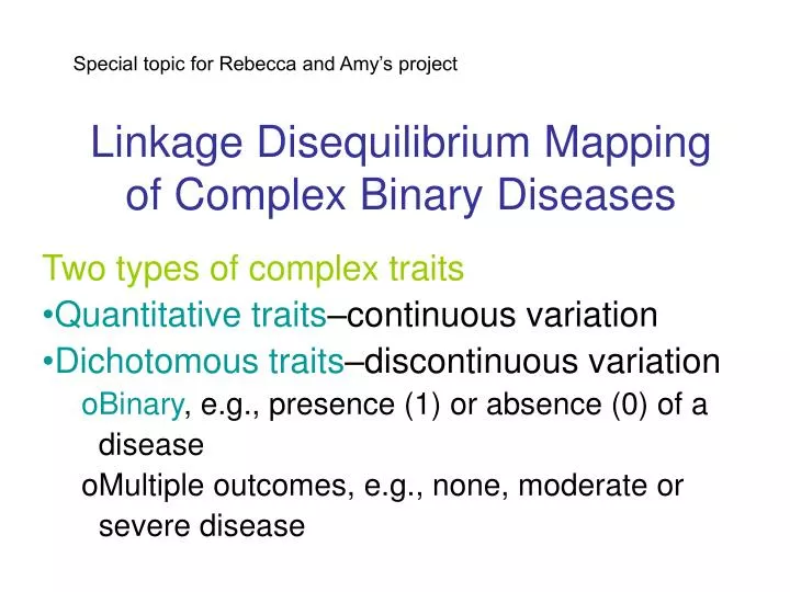
Special topic for Rebecca and Amy’s project. Linkage Disequilibrium Mapping of Complex Binary Diseases. Two types of complex traits Quantitative traits –continuous variation Dichotomous traits –discontinuous variation Binary , e.g., presence (1) or absence (0) of a disease

E N D
Special topic for Rebecca and Amy’s project Linkage Disequilibrium Mapping of Complex Binary Diseases Two types of complex traits Quantitative traits–continuous variation Dichotomous traits–discontinuous variation Binary, e.g., presence (1) or absence (0) of a disease Multiple outcomes, e.g., none, moderate or severe disease
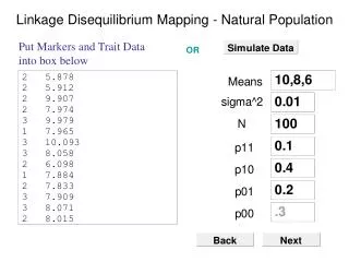
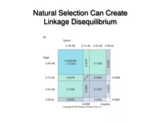
Consider a nature population • One marker with two alleles M and m, Prob(M)=p, Prob(m)=1-p • One QTL (affecting a binary trait) with two alleles A and a, Prob(A)=q, Prob(a)=1-q Four haplotypes: Prob(MQ)=p11=pq+D p=p11+p10 Prob(Mq)=p10=p(1-q)-D q=p11+p01 Prob(mQ)=p01=(1-p)q-D D=p11p00-p10p01 Prob(mq)=p00=(1-p)(1-q)+D D is the linkage disequilibrium between the marker and underlying QTL
Data structure Sample Binary (yi) Marker (j) 1 1 MM (2) 2 1 Mm (1) 3 1 Mm (1) 4 1 mm (0) 5 0 MM (2) 6 0 Mm (1) 7 0 Mm (1) 8 0 mm (0)
Arrange the data in a 2 x 3 contingency table Marker genotype 2 1 0 Affected (1) n12 n11 n10 n1. Normal (0) n02 n01 n00 n0. n.2 n.1 n.0 n Affected (1) g12 g11 g10 g1. Normal (0) g02 g01 g00 g0. g.2 g.1 g.0 1
Independence test 2df=2 = l=01j=02(nlj - mlj)2/mlj = nl=01j=02(gli - gl.g.j)2/(gl.g.j) where mlj is the expected value of nlj, mlj=ngl.g.j. H0: gli = gl.g.j H1: gli gl.g.j • Under H0, 2df=2 is central chi2-distributed for a large sample size n, with df = (2-1)x(3-1) =2 • If H0 is rejected, there is a significant D
Regression analysis Marker Model QTL model Sample Binary (yij) Marker(j) #M(Tij) There is 2 A’s 1 1 MM (2) 2 2|2 =p112 2 1 Mm (1) 1 2|1 =2p11p01 3 1 Mm (1) 1 2|1 =2p11p01 4 1 mm (0) 0 2|0 =p012 5 0 MM (2) 2 2|2 =p112 6 0 Mm (1) 1 2|1 =2p11p01 7 0 Mm (1) 1 2|1 =2p11p01 8 0 mm (0) 0 2|0 =p012 p11=pq+D, p01=(1-p)q-D
Joint and conditional (k|ij) genotype prob. between marker and QTL AA (2) Aa (1) aa (0) Obs MM p112 2p11p10 p102 n2 Mm 2p11p01 2(p11p00+p10p01) 2p10p00 n1 mm p012 2p01p00 p002 n0 MM p112 2p11p10 p102 n2 p2p2p2 Mm 2p11p01 2(p11p00+p10p01) 2p10p00 n1 2p(1-p) 2p(1-p) 2p(1-p) mm p012 2p01p00 p002 n0 (1-p)2 (1-p)2 (1-p)2
Statistical models Marker Model yij = a + bTij + ij The least squares approach can be used to estimate a and b. The size of b reflects the marker effect, confounded by the QTL effect and marker-QTL LD
The phenotype of sample i can be within marker genotype group j is modeled by yij = 1 If zij 0 If zij < where is the threshold for the underlying liability of the trait z, which is formulated as zij = ikk + eij k = the genotypic value of QTL k ik = the (1/0) indicator variable for sample i eij = normally distributed residual variable with mean 0 and variance 1
The conditional probability of yij = 1 given sample i’s QTL genotype (say Gij=k) is obtained by fk = Pr(yij=1|Gij=k,) = Pr(zij |Gij=k,) = 1 – Pr(zij < |Gij=k,) = 1 – 1/(2)-exp[-(z-k)2/2]dz fk is called the penetrance of QTL genotype k
F-values as a function of q and D Landscape F q D
Maximum likelihood analysis: Mixture model L(|y)=j=02i=0nj log [2|ijPr{yij=1|Gij=2,}yijPr{yij=0|Gij=2,}(1-yij) +1|ijPr{yij=1|Gij=1,}yijPr{yij=0|Gij=1,}(1-yij) +0|ijPr{yij=1|Gij=0,}yijPr{yij=0|Gij=0,}(1-yij)] =j=02i=0nj log[2|ijf2yij(1-f2)(1-yij)+1|ijf1yij(1-f1)(1-yij)+0|ijf0yij(1-f0)(1-yij)] = (p11, p10, p01, p00, f2, f1, f0) (6 parameters)
EM algorithm Define 2|ij= 2|ijf2yij (1-f2)(1-yij) [2|ijf2yij(1-f2)(1-yij)+1|ijf1yij(1-f1)(1-yij)+0|ijf0yij(1-f0)(1-yij)] (1) 1|ij= 1|ijf1yij (1-f1)(1-yij) [2|ijf2yij(1-f2)(1-yij)+1|ijf1yij(1-f1)(1-yij)+0|ijf0yij(1-f0)(1-yij)] (2) 0|ij= 0|ijf0yij (1-f0)(1-yij) [2|ijf2yij(1-f2)(1-yij)+1|ijf1yij(1-f1)(1-yij)+0|ijf0yij(1-f0)(1-yij)] (3) as the posterior probabilities of QTL genotypes given marker genotypes for sample i
Population genetic parameters Posterior prob AA Aa aa Obs MM 2|2i1|2i 0|2i n.2 Mm 2|1i1|1i 0|1in.1 mm 2|0i1|0i 0|0in.0 p11=1/2n{i=1n.2[22|2i+1|2i]+ i=1n.1[2|1i+1|1i] (4) p10=1/2n{i=1n.2[20|2i+1|2i]+ i=1n.1[0|1i+(1-)1|1i] (5) p01=1/2n{i=1n.0[22|0i+1|0i]+ i=1n.1[2|1i+(1-)1|1i] (6) p00=1/2n{i=1n.2[20|0i+1|0i]+ i=1n.1[0|1i+1|1i] (7)
Quantitative genetic parameters j=02i=0nj(2|ijyij) f2 = (8) j=02i=0nj 2|ij j=02i=0nj(1|ijyij) f1 = (9) j=02i=0nj 1|ij j=02i=0nj(0|ijyij) f0 = (10) j=02i=0nj 0|ij
EM algorithm (1) Give initiate values (0) =(p11,p10,p01,p00,f2,f1,f0)(0) (2) Calculate 2|ij(1), 1|ij(1)and 0|ij(1)using Eqs. 1-3, (3) Calculate (1) using 2|ij(1), 1|ij(1)and 0|ij(1)based on Eqs. 4-10, (4) Repeat (2) and (3) until convergence.
Three genotypic values 2 = + a for AA 1 = + d for Aa 0 = - a for aa With the MLEs of k, we can estimate , a and d.
How to estimate k? f2 = 1 – 1/(2)-exp[-(z-2)2/2]dz f1 = 1 – 1/(2)-exp[-(z-1)2/2]dz f0 = 1 – 1/(2)-exp[-(z-0)2/2]dz We can use numerical approaches to estimate 2,1 and 0
Hypothesis test H0: f2 = f1 = f0 H1: at least one equality does not hold LR = -2[logL(0|y,M,D) - logL(1|y,M,D)] for interval [max{-p(1-q),-(1-p)q}, min{pq, (1-p)(1-q)}] of D. 0 = MLE under H0 1 = MLE under H1
LR as a function of D Profile D min{p(1-q),(1-p)q} max{pq.(1-p)(1-q)}