Download
1 / 24
240 likes | 355 Vues
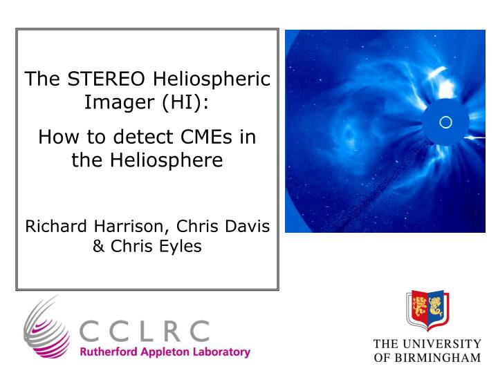
The STEREO Heliospheric Imager (HI): How to detect CMEs in the Heliosphere Richard Harrison, Chris Davis & Chris Eyles.

E N D
The STEREO Heliospheric Imager (HI): How to detect CMEs in the Heliosphere Richard Harrison, Chris Davis & Chris Eyles
First opportunity to observe geoeffective CMEs along the Sun-Earth line in interplanetary space - the first instrument to detect CMEs in a field of view including the Earth! • First opportunity to obtain stereographic views of CMEs in interplanetary space - to investigate CME structure, evolution and propagation • Method: Occultation and baffle system, with wide angle view of the heliosphere, achieving light rejection levels of 3x10-13 and 10-14 of the solar brightness
The HI Basic Design Radiator HI-1 Door Side & rear baffles Door latch mechanism HI-2 Inner Baffles Forward Baffles Direction of Sunlight
HI Basic Design/Operation • Geometrical Requirements: To view the Sun-Earth line with unbroken coverage from corona to Earth orbit Opening angle of 45 degrees governed by average CME width over equator • Brightness Levels: Need to achieve rejection to < 3x10-13 & < 10-14 B/Bo to detect CME signal Have to contend with contributions from the F-corona, planets, stars, the Earth and Moon
HI Consortium HI Principal Investigator R. Harrison (RAL) SECCHI/NRL PPARC Instrument Manager C. Eyles (Birmingham) CCD Camera Lead Engineer N. Waltham (RAL) CSL Lead J.-M. Defise (CSL) CCD Camera Scientist J. Lang (RAL) HI Straylight Design J.P. Halain (CSL) HI Optical Design E. Mazy (CSL) Thermal Design H. Mapson-Menard (B’ham) Mechanical Design C. Longstaff (B’ham) Mechanical Workshop A. Jones (B’ham) Structural Analysis H. Mapson-Menard (B’ham) Electronics Design D. Hoyland (B’ham) Contamination Control & QA D. Smith (B’ham)
HI – Image Simulation HI image simulation activity - started in Autumn 2002. See ‘Image Simulations for the Heliospheric Imager’, C. J. Davis & R.A. Harrison, available at http://www.stereo.rl.ac.uk.
HI – Image Simulation • Purpose: • To assess the impact of all sources and effects, including saturation, non-shutter operation etc… • To investigate image processing requirements for, e.g. cosmic ray correction, F-corona & stellar subtraction techniques, and other techniques for the extraction of CME and other science data. • To provide a tool to explore operations scenarios with the user community. In addition to demonstrating that HI works, and exploring the ways we can use it, the simulation provides requirements to the on-board and ground software efforts, to operations planning etc...
HI – Image Simulation 1. The F-coronal intensity Calculated from Koutchmy & Lamy, 1985 - plotted below for HI-1 and HI-2, along ecliptic.
HI – Image Simulation 2. The Planets Include 4 brightest planets at their maximum intensity. Venus Jupiter F-corona Intensity vs elongation (pixel number), including two planets - nominal HI-2 60 s exposure.
HI – Image Simulation 3. The HI Point Spread Function All contributions modelled (including design, lens location tolerance, lens manufacture, surface form, CCD axial position accuracy etc…): HI-1 & HI-2 RMS spot diameters = 45 to 66 μm (3.3 to 4.9 pix) & 105 to 145 μm (7.8 to 10.7 pix). Note - Pixel size = 13.5 micron. The HI Image Simulation analysis assumes a Gaussian of width 50 and 100 μm for HI-1 and HI-2 respectively. 4. Noise Included as a Poisson-like distribution using the IDL ‘randomn’ function applied to each pixel.
HI – Image Simulation 5. Stray Light To mimic the anticipated stray light contribution, the HI Simulation analysis uses the CSL forward baffle mock up tests (May 2002) including a 10-4 rejection from the lens-barrel assemblies.
HI – Image Simulation 6. Stars We require a distribution of point-like sources to mimic the stellar distribution - use C.W. Allen (Astrophysical Quantities) for stellar density as a function of magnitude. Red entries are those that saturate.
HI – Image Simulation 6. Stars (continued) HI-2 nominal 60 s exposure shown as several superimposed slices across CCD. Includes stars to 12th mag, four planets, F-corona and stray light. The PSF is applied. This illustrates the impact of the stellar distribution!
HI – Image Simulation • 7. Saturation and Blooming • The CCD pixels saturate at 200,000 electrons (full well). At DQE of 0.8 that is 250,000 photons. When pixels saturate excess charge spills into adjacent pixels (blooming). Images can be swamped, by sources of excessive brightness. • HI must detect brightness levels down to 10-13 to 10-14 Bsun; we know that sources will saturate. • Aim: Minimise effect - restrict blooming to columns which include the bright source. • Tests confirm - detector saturation is confined to columns. For the simulation, first the PSF is applied, then blooming is calculated by distributing excess charge up and down the relevant columns. Test data: 512 ms exposure producing saturation factor of 764 - equivalent to Jupiter in HI-1.
HI – Image Simulation CCD Saturation F-corona, stray light, plus stellar & planetary ‘background’, with PSF and noise applied
HI – Image Simulation 8. Line Transfer Function (non-shutter operation) HI does not have a shutter. The CCD is read out from the bottom. Consider one pixel (n,m) - its nominal exposure is made at location (n,m). After the image is exposed, a line transfer process carries the image down the column at a rate of 2048 μs per line - thus we must add (m-1) exposures of 2048 μs to the nominal exposure. After reading out the CCD, it is ‘cleared’ at a rate of 150 μs per line - i.e. the (2048-m) locations ‘above’ the location (n,m) contribute 150 μs exposures. nth column 2048 pixels Pixel (n,m) Readout direction 2048 pixels
HI – Image Simulation 8. Line Transfer Function (non-shutter operation) (continued) The HI simulated images are being used to investigate the effect of non-shutter operation. This allows a comparison of the shutter and non-shutter exposures. We can take steps to correct for this. A South to North cut of intensity across a nominal HI-2 image showing the effect of non-shutter (upper curve) and shutter (lower curve).
HI – Image Simulation • 9. Cosmic Rays • Cosmic ray hits will be a significant effect. The SOHO CCD hit data from Pike & Harrison (2000) are taken - assuming 4 hits/cm2s - i.e. 30.5 hits per second on each of the HI CCDs. • Cosmic ray are considered to have variable intensities and leave tracks depending on their direction of arrival (considered to be equally likely from any direction). The active depth of the HI CCDs (10 microns) means that long tracks are unlikely but possible. • Cosmic rays must be extracted, during nominal operations, after each exposure, on board. Simulated exposures for each instrument are being used to test the on-board extraction codes. Can these be extracted without removing the faint signatures of Near Earth Objects (NEOs)?
HI2 – Earth-Moon Occulter • 10. Earth Occulter • The brightness of the Earth in the early phase of the mission is such that the HI-2 image would saturate (the Earth’s intensity would be 1,250,000 times the pixel saturation level at mission start) • We must occult the Earth until its intensity is about that of Venus
HI – Image Simulation The story so far... HI-2 Simulated Image - nominal exposure (60 s) - non-shutter effect included. Planets F-corona & stray light HI2 Occulter Stellar ‘background’ down to 13th mag. Saturation of brightest planets & stars HI Point Spread Function & noise included. Not included: Earth/Moon Cosmic rays
HI – Image Simulation 10. And finally… A CME! The simulation currently includes a simple semi-circular CME of rather weak intensity (Socker et al. 2000) - where??? Base-frame subtraction methods (to remove F-corona & stellar background), & image subtraction, are under investigation. The simulation activity is providing requirements on the ground software which is being developed. The unique aspect of HI is the need to subtract carefully the stellar contribution.
HI – Image Simulation Image with base-frame subtracted - revealing dummy CME loop
Conclusions The simulation activity includes all known effects and demonstrates how the HI instruments can be used to detect and analyse CMEs in the heliosphere – thus with the launch of STEREO we will see a new chapter in the study of Earth-directed CMEs, the propagation of CMEs and CME 3D structure.