Download
1 / 44
450 likes | 639 Vues
Pitch Tracking + Prosody. January 17, 2012. The Plan for Today. One announcement: On Thursday, we’ll meet in the Craigie Hall D 428 We’ll be working on intonation transcription… The plan for today: Wrap up A-to-D conversion Automatic Pitch Tracking (Brief) suprasegmentals review

E N D
Pitch Tracking + Prosody January 17, 2012
The Plan for Today • One announcement: • On Thursday, we’ll meet in the Craigie Hall D 428 • We’ll be working on intonation transcription… • The plan for today: • Wrap up A-to-D conversion • Automatic Pitch Tracking • (Brief) suprasegmentals review • The basics of English intonation
Sample Size Demo • 11k 16 bits • 11k 8 bits • 8k 16 bits • 8k 8bits (telephone) • Note: CDs sample at 44,100 Hz and have 16-bit quantization. • Also check out bad and actedout examples in Praat. • Also: look at Praat’s representation of a .sound file.
Quantization Range • With 16-bit quantization, we can encode 65,536 different possible amplitude values. • Remember that I(dB) = 10 * log10 (A2/r2) • Substitute the max and min amplitude values for A and r, respectively, and we get: • I(dB) = 10 * log10 (655362/12) = 96.3 dB • Some newer machines have 24-bit quantization-- • = 16,777,216 possible amplitude values. • I(dB) = 10 * log10 (167772162/12) = 144.5 dB • This is bigger than the range of sounds we can listen to without damaging our hearing.
Problem: Clipping • Clipping occurs when the pressure in the analog signal exceeds the sample size range in digitization • Check out sylvester and normal in Praat.
A Note on Formats • Digitized sound files come in different formats… • .wav, .aiff, .au, etc. • Lossless formats digitize sound in the way I’ve just described. • They only differ in terms of “header” information and specified limits on file size, etc. • Lossy formats use algorithms to condense the size of sound files • …and the sound file loses information in the process. • For instance: the .mp3 format primarily saves space by eliminating some very high frequency information. • (which is hard for people to hear)
AIFF vs. MP3 .aiff format .mp3 format (digitized at 128 kB/s) • This trick can work pretty well…
MP3 vs. MP3 .mp3 format (digitized at 128 kB/s) .mp3 format (digitized at 64 kB/s) • .mp3 conversion can induce reverb artifacts, and also cut down on temporal resolution (among other things).
Sound Digitization Summary • Samples are taken of an analog sound’s pressure value at a recurring sampling rate. • This digitizes the time dimension in a waveform. • The sampling frequency needs to be twice as high as any frequency components you want to capture in the signal. • E.g., 44100 Hz for speech • Quantization converts the amplitude value of each sample into a binary number in the computer. • This digitizes the amplitude dimension in a waveform. • Rounding off errors can lead to quantization noise. • Excessive amplitude can lead to clipping errors.
The Digitization of Pitch • Praat can give us a representation of speech that looks like: • The blue line represents the fundamental frequency (F0) of the speaker’s voice. • Also known as a pitch track • How can we automatically “track” F0 in a sample of speech?
Pitch Tracking • Voicing: • Air flow through vocal folds • Rapid opening and closing due to Bernoulli Effect • Each cycle sends an acoustic shockwave through the vocal tract • …which takes the form of a complex wave. • The rate at which the vocal folds open and close becomes the fundamental frequency (F0) of a voiced sound.
Voicing Bars Individual glottal pulses
Voicing = Complex Wave • Note: voicing is not perfectly periodic. • …always some random variation from one cycle to the next. • How can we measure the fundamental frequency of a complex wave?
duration = ??? • The basic idea: figure out the period between successive cycles of the complex wave. • Fundamental frequency = 1 / period
Measuring F0 • To figure out where one cycle ends and the next begins… • The basic idea is to find how well successive “chunks” of a waveform match up with each other. • One period = the length of the chunk that matches up best with the next chunk. • Automatic Pitch Tracking parameters to think about: • Window size (i.e., chunk size) • Step size • Frequency range (= period range)
Window (Chunk) Size Here’s an example of a small window
Window (Chunk) Size Here’s an example of a large(r) window
Initial window of the waveform is compared to another window (of the same duration) at a later point in the waveform
Matching ??? The waveforms in the two windows are compared to see how well they match up. Correlation = measure of how well the two windows match
Autocorrelation • The measure of correlation = • Sum of the point-by-point products of the two chunks. • The technical name for this is autocorrelation… • because two parts of the same wave are being matched up against each other. • (“auto” = self)
Autocorrelation Example • Ex: consider window x, with n samples… • What’s its correlation with window y? • (Note: window y must also have n samples) • x1 = first sample of window x • x2 = second sample of window x • … • xn = nth (final) sample of window x • y1 = first sample of window y, etc. • Correlation (R) = x1*y1 + x2* y2 + … + xn* yn • The larger R is, the better the correlation.
By the Numbers • Sample 1 2 3 4 5 6 • x .8 .3 -.2 -.5 .4 .8 • y -.3 -.1 .1 .3 .1 -.1 • product -.24 -.03 -.02 -.15 .04 -.08 • Sum of products = -.48 • These two chunks are poorly correlated with each other.
By the Numbers, part 2 • Sample 1 2 3 4 5 6 • x .8 .3 -.2 -.5 .4 .8 • z .7 .4 -.1 -.4 .1 .4 • product .56 .12 .02 .2 .04 .32 • Sum of products = 1.26 • These two chunks are well correlated with each other. • (or at least better than the previous pair) • Note: matching peaks count for more than matches close to 0.
Back to (Digital) Reality ??? These two windows are poorly correlated The waveforms in the two windows are compared to see how well they match up. Correlation = measure of how well the two windows match
Next: the pitch tracking algorithm moves further down the waveform and grabs a new window
“step” The distance the algorithm moves forward in the waveform is called the step size
Matching, again ??? The next window gets compared to the original.
Matching, again ??? These two windows are also poorly correlated The next window gets compared to the original.
another “step” The algorithm keeps chugging and, eventually…
Matching, again ??? These two windows are highly correlated The best match is found.
period The fundamental period can be determined by the calculating the length of time between the start of window 1 and the start of (well correlated) window 2.
Mopping up period • Frequency is 1 / period • Q: How many possible periods does the algorithm need to check? • Frequency range (default in Praat: 75 to 600 Hz)
Moving on • Another comparison window is selected and the whole process starts over again.
The algorithm ultimately spits out a pitch track. • This one shows you the F0 value at each step. would I like Uhm A flight to Seattle from Albuquerque Thanks to Chilin Shih for making these materials available
Pitch Tracking in Praat • Play with F0 range. • Create Pitch Object. • Also go To Manipulation…Pitch. • Also check out:
Summing Up • Pitch tracking uses three parameters • Window size • Ensures reliability • In Praat, the window size is always three times the longest possible period. • E.g.: 3 X 1/75 = .04 sec. • Step size • For temporal precision • Frequency range • Reduces computational load
Deep Thought Questions • What might happen if: • The shortest period checked is longer than the fundamental period? • AND two fundamental periods fit inside a window? • Potential Problem #1: Pitch Halving • The pitch tracker thinks the fundamental period is twice as long as it is in reality. • It estimates F0 to be half of its actual value
Pitch Halving pitch is halved Check out normal file in Praat.
More Deep Thoughts • What might happen if: • The shortest period checked is less than half of the fundamental period? • AND the second half of the fundamental cycle is very similar to the first? • Potential Problem #2: Pitch doubling • The pitch tracker thinks the fundamental period is half as long as it actually is. • It estimates the F0 to be twice as high as it is in reality.
Pitch Doubling pitch is doubled
Microperturbations • Another problem: • Speech waveforms are partly shaped by the type of segment being produced. • Pitch tracking can become erratic at the juncture of two segments. • In particular: • voiced to voiceless segments • sonorants to obstruents • These discontinuities in F0 are known as microperturbations. • Also: transitions between modal and creaky voicing tend to be problematic.
Back to Language • F0 is important because it can be used by languages to signal differences in meaning. • Note: • Acoustic = Fundamental Frequency • Perceptual = Pitch • Linguistic = Tone
A Typology • F0 is generally used in three different ways in language: 1. Tone languages (Chinese, Navajo, Igbo) • Lexically determined tone on every syllable • “Syllable-based” tone languages 2. Accentual languages (Japanese, Swedish) • The location of an accent in a particular word is lexically marked. • “Word-based” tone languages 3. Stress languages (English, Russian) • It’s complicated.