Download
1 / 65
650 likes | 654 Vues
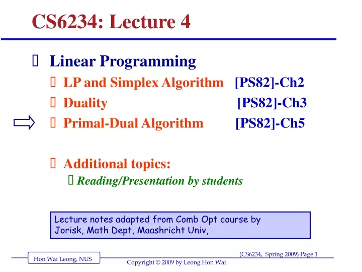
CS6234: Lecture 4. Linear Programming LP and Simplex Algorithm [PS82]-Ch2 Duality [PS82]-Ch3 Primal-Dual Algorithm [PS82]-Ch5 Additional topics: Reading/Presentation by students. Lecture notes adapted from Comb Opt course by Jorisk, Math Dept, Maashricht Univ,.

E N D
CS6234: Lecture 4 • Linear Programming • LP and Simplex Algorithm [PS82]-Ch2 • Duality [PS82]-Ch3 • Primal-Dual Algorithm [PS82]-Ch5 • Additional topics: • Reading/Presentation by students Lecture notes adapted from Comb Opt course by Jorisk, Math Dept, Maashricht Univ,
Combinatorial Optimization Chapter 5 [PS82] The primaldual algorithm Combinatorial Optimization Masters OR
Primal Dual Method found x, succeed! primal dual restricted primal restricted dual Source: CUHK, CS5160 y z Construct a better dual Combinatorial Optimization Masters OR
LP in standard form + Dual Primal min c’ x s.t. A x = b (≥ 0 )(P) x ≥ 0 maxπ’ b s.t. π’A ≤ c (D) π’free Dual Combinatorial Optimization Masters OR
Definition of the Dual Definition 3.1: Given an LP in general form, called the primal, the dual is defined as follows Combinatorial Optimization Masters OR
Complementary slackness Theorem 3.4 A pair, x, π, respectively feasible in a primal-dual pair is optimal if and only if: ui = πi(a’ix - bi) = 0 for all i (1) vj = (cj - π’Aj)xj= 0 for all j. (2) Combinatorial Optimization Masters OR
Idea of a Primal-Dual Algorithm Suppose we have a dual feasible solution π. If we can find a primal feasible solution x such that xj= 0 whenever cj – π’Aj > 0 then: Aix = bi for all i and hence (1) holds because x is a feasible solution to the primal (2) holds because xj = 0 whenever cj – π’Aj = 0. Thus the complementary slackness relations hold, and hence x and πare optimal solutions to the primal problem (P) and the dual problem (D) resp. Combinatorial Optimization Masters OR
Outline of the primal dual algorithm P D RP DRP x ρ π Adjustment to π Combinatorial Optimization Masters OR
Primal Dual Method found x, succeed! primal dual restricted primal restricted dual Source: CUHK, CS5160 y z Construct a better dual Combinatorial Optimization Masters OR
Getting started: finding a dual feasible π If c ≥ 0,π = 0 is a dual feasible solution. When cj < 0 for some j, introduce variable xm+1, and the additional constraint x1 + x2 + … + xm+1 = bm+1. (bm+1large enough) The dual (D) then becomes maxπ’ b + πm+1 bm+1 s.t. π’A + πm+1 ≤ cjfor all j, πm+1 ≤ 0. The solution πi = 0, i=1…m, and πm+1 = minj cj < 0 is feasible for the dual (D). Combinatorial Optimization Masters OR
Given a dual feasible solution π Thus, we assume we have a dual feasible solution π. Consider the set J = { j : π’j Aj = cj }. A solution x to the primal (P) is optimal iffxj=0 for all j not in J. Hence, we aim for an x feasible in Σj=1n aij xj = bi i =1,..,m xj ≥ 0, for all j in J xj = 0, for all j not in J Combinatorial Optimization Masters OR
Restricted Primal (RP) Min ξ = Σj=1m xja Σj=1n aijxj + xja= bi i =1,..,m xj ≥ 0, for all j in J (RP) xj = 0, for all j not in J xja≥ 0, i =1,..,m If ξopt = 0, the corresponding optimal solution to (RP) yields an x which satisfies (together with π)the complementary slackness conditions. Thus, in the remainder we consider the case where ξopt > 0. Combinatorial Optimization Masters OR
The dual of the restricted primal:DRP Min Σj=1m xja s.t. ΣjεJ aij xj+ xja= bi i =1,..,m xj ≥ 0, for all j in J (RP) xj = 0, for all j not in J xja≥ 0, i =1,..,m Maxπ’ b s.t. π’Aj ≤ 0 for all j in J πi ≤ 1, i=1…m, πifree i=1…m, We denote by ρ the optimal solution of this (DRP). Combinatorial Optimization Masters OR
(D) Maxπ’ b s.t. π’Aj ≤ cjj=1…n πi free i=1…m. (DRP) Maxπ’ b s.t. π’Aj ≤ 0 for all j in J πi ≤ 1, i=1…m, πifree i=1…m. Comparison of (D) and (DRP) Combinatorial Optimization Masters OR
A Primal Dual iteration…. Let θε R, and consider π* =π +θρ. Assume θ is such that π* is feasible in (D). Then π*’ b =π’b+θρ’b. Obviously ρ’b = ξopt > 0, since otherwise x together with πsatisfiesthe complementary slackness conditions. Thus, by choosing θ > 0, π*’ b >π’b, yielding an improved solution of the dual (D). Combinatorial Optimization Masters OR
A Primal Dual iteration Forπ* to be feasible in (D), it must hold that: π*’Aj =π’Aj +θρ’Aj ≤ cj , j=1…n. From the definition of (DRP) it holds that ρ’Aj ≤ 0 for all j in J. Thus if ρ’Aj ≤ 0 for all j, we can choose θ = +∞.But then (D) is unbounded, and hence (P) is infeasible. (Theorem 5.1) Thus, we assume that ρ’Aj > 0 for some j not in J. Combinatorial Optimization Masters OR
A Primal Dual iteration We are going to allow j to ‘enter the basis’ of (D)… Let θ1to be the maximum value such that π’ Aj+ θρ’Aj ≤ cj for all j not in J and ρ’Aj > 0 Define π* = π +θ1 ρ. Then π*’b =π’ b+θ1 ρ’ b > π*’b. Dual constraint j is satisfied at equality, and then by complementary slackness, primal variable xj can have nonnegative value Combinatorial Optimization Masters OR
The Primal Dual Algorithm Input: Feasible solution πfor (D). Output: Optimal solution x for (P) if it exists. Infeasible false; opt false; While not (infeasible or opt) begin J {j: π’Aj =cj } Solve (RP) giving solution x. Ifξopt = 0 then opt true else ifρ’A ≤ 0 then infeasible true elseππ + θ1 ρ End {while} Combinatorial Optimization Masters OR
Admissible columns Definition Given a solution π to the dual (D), let J ={ j : π’Aj =cj }. Then any column Aj , jεJ is called an admissable columns. Theorem 5.3. A column which is in the optimal basis of (RP) and admissable in some iteration of the Primal Dual algorithm remains admissable at the start of the next iteration. Combinatorial Optimization Masters OR
Admissable columns Proof. If Aj is in the optimal basis of (RP) then, by complementary slackness dj - ρ’Aj = 0, where dj is the cost coefficient in the objective function of the (RP). Hence dj= 0, and thus ρ’Aj = 0. This in turn implies that π*’ Aj = π’ Aj+ θρ’Aj = π’ Aj = cj Since j was an admissable column. Thus j remains an admissable column. Combinatorial Optimization Masters OR
Consequence In each iteration, the optimal solution x of (RP), is also a basic feasible solution of the (RP) in the next iteration. Thus subsequent (RP)’s can be solved taking the optimal solution of the previous one as a starting point for a simplex iteration. Moreover, using an anti cycling rule, the Primal Dual algorithm is finite (see Theorem 5.4). Combinatorial Optimization Masters OR
A Primal Dual method for Shortest Path node-arc incidence matrix A: 1 if arc k leaves node i aij= { -1 if arc k enters node i 0 otherwise Primal (P): min c’ f s.t. Σk Ak fk = 0 for all i ≠ s,t. Σk Ak fk = 1 i = s. f ≥ 0 Combinatorial Optimization Masters OR
Dual (D) of the shortest path problem max πs s.t. πi - πj ≤ cij, πfree, πt = 0. Admissable arcs J ={ arcs (i,j) : πi - πj = cij }. Combinatorial Optimization Masters OR
Restricted Primal (RP) of Shortest Path min Σi xia s.t. ΣkεJ Ak fk + xia= 0 for all i ≠ s,t. Σ{j:(s,j)εJ} A(s,j)f(s,j) + xsa = 1 fk ≥ 0 for all k, fk = 0 for all k not in J, xia ≥ 0 for all i. Combinatorial Optimization Masters OR
Dual of the Restricted Primal (DRP) max πs s.t. πi - πj ≤ 0, for all arcs (i,j) in J. πi ≤ 1, for all i. πt = 0, πfree, Combinatorial Optimization Masters OR
Solving (DRP) Obviously πs ≤ 1, and since we aim to maximize πs we try πs = 1. But then all nodes i reachable by an admissable arc from s must also have πi = 1. This argument applies recursively. Similarly since πt = 0, all nodes i (recursively) reachable from the sink, must have πi = 0. Combinatorial Optimization Masters OR
Optimal solution ρ to (DRP) If the source can be reached from the sink by a path consisting of admissable arcs πs = 1 end hence (RP) has optimal value zero and we are done. t 1 1 0 s Combinatorial Optimization Masters OR
Solving (DRP) Let θ1to be the maximum value such that π’ Ak+ θρ’Ak≤ ck for all k not in J and ρ’Ak > 0. Thus we must consider (i,j) such that ρi -ρj =1. Therefore θ1is the minimum over the aforementioned (i,j) of cij – (πi -πj ). Interpretation on next slide… Combinatorial Optimization Masters OR
Interpretation of Primal Dual iteration We assume cij > 0 for i,j = 1…m. Then the solution πi = 0 for i=1…m is feasible in (D), and selected as the starting solution. We select a non admissable arc from a green or red node i (which has ρi = 1 to a yellow node j, which has ρi = 0. Since arc (i,j) is non admissable it must hold that πi – πj < cij. Combinatorial Optimization Masters OR
Example 3 1 3 2 2 t 3 s 2 5 1 4 2 1 Combinatorial Optimization Masters OR
Initial dual feasible solution π1=0 π3=0 3 1 3 2 2 πt=0 πs=0 t 3 s 2 5 1 4 2 1 π4=0 π2=0 Admissable arcs: Ø Combinatorial Optimization Masters OR
Initial solution of (RP) xsa=1, xia=0, for all i ≠ s, no variables fkfor admissable columns Ak. Combinatorial Optimization Masters OR
First DRP ρ1=1 ρ3=1 3 1 3 2 2 ρt=0 ρs=1 t 3 s 2 5 1 4 2 1 ρ4=1 ρ2=1 θ1 = c3t + πt - π3= 2 Combinatorial Optimization Masters OR
Next solution of (RP) xsa=1, xia=0, for all i ≠ s, variables fkfor admissable columns Akfrom node 3 to t, but primal variables remain unchanged. (and will remain unchanged, until some arc leaving s is admissable… Combinatorial Optimization Masters OR
Next dual feasible solution π1=2 π3=2 3 1 3 2 2 πt=0 πs=2 t 3 s 2 5 1 4 2 1 π4=2 π2=2 Admissable arcs: (3,t) Combinatorial Optimization Masters OR
Next DRP ρ1=1 ρ3=0 3 1 3 2 2 ρt=0 ρs=1 t 3 s 2 5 1 4 2 1 ρ4=1 ρ2=1 θ1 = c43 + π3 -π4 = 2 Combinatorial Optimization Masters OR
Next dual feasible solution π1=4 π3=2 3 1 3 2 2 πt=0 πs=4 t 3 s 2 5 1 4 2 1 π4=4 π2=4 Admissable arcs: (3,t), (4,3) Combinatorial Optimization Masters OR
Next DRP ρ1=1 ρ3=0 3 1 3 2 2 ρt=0 ρs=1 t 3 s 2 5 1 4 2 1 ρ4=0 ρ2=1 θ1 = c24 + π4 -π2 = 1 = c13 + π3 -π1 = 1 Combinatorial Optimization Masters OR
Next dual feasible solution π1=5 π3=2 3 1 3 2 2 πt=0 πs=5 t 3 s 2 5 1 4 2 1 π4=4 π2=5 Admissable arcs: (3,t), (4,3), (1,3), (2,4) Combinatorial Optimization Masters OR
Next DRP ρ1=0 ρ3=0 3 1 3 2 2 ρt=0 ρs=1 t 3 s 2 5 1 4 2 1 ρ4=0 ρ2=0 θ1 = cs2 + π2 -πs = 1 Combinatorial Optimization Masters OR
Next dual feasible solution π1=5 π3=2 3 1 3 2 2 πt=0 πs=6 t 3 s 2 5 1 4 2 1 π4=4 π2=5 Admissable arcs: (3,t), (4,3), (1,3), (2,4),(s,2) Combinatorial Optimization Masters OR
Next solution of (RP) xia=0, for all i, fs2=1, f24=1, f43=1, f3t=1, all other fij = 0. Solution value 0 f is feasible in primal (P), and since c ’x = π’b optimal in (P)! Combinatorial Optimization Masters OR
Combinatorialization… (P) has an integer cost vector c, and (0,1) right hand side. (RP) has a (0,1) cost vector and right hand side b. Therefore in (RP) the complexity is not from the numbers but from the combinatorics. Similarly (D) has a (0,1) vector b, and integer right hand side c. (DRP) has a (0,1) cost vector and right hand side. Therefore in (DRP) the complexity is not from the numbers but from the combinatorics. The primal dual algorithm solves a problem with ‘numerical’ complexity, by repeatedly solving a problem which has only ‘combinatorial’ complexity. This concept, which Papadimitriou calls ‘combinatorialization’ is frequently encountered in combinatorial optimization. Combinatorial Optimization Masters OR
Primal Dual Method found x, succeed! primal dual restricted primal restricted dual Lecture 20: March 28 y z Construct a better dual
Primal Dual Program Primal Program Dual Program If there is a feasible primal solution x and a feasible dual solution y, then both are optimal solutions. Primal-Dual Method: An algorithm to construct such a pair of solutions.
Optimality Condition Suppose there is a feasible primal solution x, and a feasible dual solution y. How do we check that they are optimal solutions? Avoid strict inequality
Optimality Condition Avoid strict inequality
Complementary Slackness Conditions Primal complementary slackness condition: Dual complementary slackness condition:
Primal Dual Method Start from a feasible dual solution. Search for a feasible primal solution satisfying complementary slackness conditions. If not, improve the objective value of dual solution. repeat